Combining (lots of) numerical and categorical predictors

ANCOVAs and beyond

Remember you should

• add code chunks by clicking the Insert Chunk button on the toolbar or by pressing Ctrl+Alt+I to answer the questions!
• use visual mode or render your file to produce a version that you can see!
• render your file to make sure it runs (and that you haven’t been working out of order)
• save your work often
  • commit it via git!
  • push updates to github

Example

Following the iris example from class

set.seed(3)
iris_example_species <-data.frame(
  Species = c(rep("baruch",25), rep("hunter", 25), rep("york", 25)),
  Petal_Length = runif(75,2,4 ))
set.seed(31)
iris_example_species$Sepal_interaction <- 
  iris_example_species$Petal_Length * c(rep(-2, 25),rep(0,25), rep(5,25)) + 
  c(rep(2,25), rep(3,25), rep(4,25)) + rnorm(75)

Plot the data

library(ggplot2)
ggplot(iris_example_species, aes(x= Petal_Length, y = Sepal_interaction, color = Species)) +
  geom_point()+
  ylab("Sepal Length") +
  xlab("Petal Length") +
  ggtitle("Impact of petal length and species on sepal length") +
    geom_smooth(method = "lm", se = F)

`geom_smooth()` using formula = 'y ~ x'

Analysis would indicate (assumption plots not shown here to allow focus on interpreting interactions)

library(car)
Anova(lm( Sepal_interaction~ Petal_Length * Species, iris_example_species), 
      type = "III")

Anova Table (Type III tests)

Response: Sepal_interaction
                      Sum Sq Df  F value    Pr(>F)    
(Intercept)            7.076  1   8.0267  0.006038 ** 
Petal_Length          38.452  1  43.6177  6.88e-09 ***
Species                3.353  2   1.9015  0.157092    
Petal_Length:Species 227.334  2 128.9368 < 2.2e-16 ***
Residuals             60.828 69                       
---
Signif. codes:  0 '***' 0.001 '**' 0.01 '*' 0.05 '.' 0.1 ' ' 1

interactions do exist. This means we can’t interpret the “general” relationship, so we need to look for each species using regression.

summary(lm(Sepal_interaction ~ Petal_Length, 
         iris_example_species[iris_example_species$Species == "baruch",]))

Call:
lm(formula = Sepal_interaction ~ Petal_Length, data = iris_example_species[iris_example_species$Species == 
    "baruch", ])

Residuals:
    Min      1Q  Median      3Q     Max 
-1.7194 -0.5504 -0.1860  0.4736  1.7067 

Coefficients:
             Estimate Std. Error t value Pr(>|t|)    
(Intercept)    2.9734     0.9767   3.044  0.00576 ** 
Petal_Length  -2.3663     0.3335  -7.097 3.14e-07 ***
---
Signif. codes:  0 '***' 0.001 '**' 0.01 '*' 0.05 '.' 0.1 ' ' 1

Residual standard error: 0.8738 on 23 degrees of freedom
Multiple R-squared:  0.6865,    Adjusted R-squared:  0.6728 
F-statistic: 50.36 on 1 and 23 DF,  p-value: 3.144e-07

Anova(lm(Sepal_interaction ~ Petal_Length, 
         iris_example_species[iris_example_species$Species == "baruch",]), 
      type="III")

Anova Table (Type III tests)

Response: Sepal_interaction
             Sum Sq Df F value    Pr(>F)    
(Intercept)   7.076  1  9.2676  0.005758 ** 
Petal_Length 38.452  1 50.3604 3.144e-07 ***
Residuals    17.561 23                      
---
Signif. codes:  0 '***' 0.001 '**' 0.01 '*' 0.05 '.' 0.1 ' ' 1

summary(lm(Sepal_interaction ~ Petal_Length, 
           iris_example_species[iris_example_species$Species == "hunter",]))

Call:
lm(formula = Sepal_interaction ~ Petal_Length, data = iris_example_species[iris_example_species$Species == 
    "hunter", ])

Residuals:
     Min       1Q   Median       3Q      Max 
-1.89221 -0.58055  0.00876  0.47006  2.49756 

Coefficients:
             Estimate Std. Error t value Pr(>|t|)
(Intercept)    1.2564     1.1463   1.096    0.284
Petal_Length   0.4962     0.3895   1.274    0.215

Residual standard error: 0.9902 on 23 degrees of freedom
Multiple R-squared:  0.06589,   Adjusted R-squared:  0.02528 
F-statistic: 1.622 on 1 and 23 DF,  p-value: 0.2155

Anova(lm(Sepal_interaction ~ Petal_Length, 
         iris_example_species[iris_example_species$Species == "hunter",]), 
      type="III")

Anova Table (Type III tests)

Response: Sepal_interaction
              Sum Sq Df F value Pr(>F)
(Intercept)   1.1779  1  1.2014 0.2844
Petal_Length  1.5907  1  1.6224 0.2155
Residuals    22.5503 23               

summary(lm(Sepal_interaction ~ Petal_Length, 
           iris_example_species[iris_example_species$Species == "york",]))

Call:
lm(formula = Sepal_interaction ~ Petal_Length, data = iris_example_species[iris_example_species$Species == 
    "york", ])

Residuals:
     Min       1Q   Median       3Q      Max 
-1.45150 -0.69660  0.02717  0.83006  1.64698 

Coefficients:
             Estimate Std. Error t value Pr(>|t|)    
(Intercept)    4.0617     0.9550   4.253    3e-04 ***
Petal_Length   4.9642     0.3024  16.417  3.4e-14 ***
---
Signif. codes:  0 '***' 0.001 '**' 0.01 '*' 0.05 '.' 0.1 ' ' 1

Residual standard error: 0.9491 on 23 degrees of freedom
Multiple R-squared:  0.9214,    Adjusted R-squared:  0.918 
F-statistic: 269.5 on 1 and 23 DF,  p-value: 3.401e-14

Anova(lm(Sepal_interaction ~ Petal_Length, 
         iris_example_species[iris_example_species$Species == "york",]), 
      type="III")

Anova Table (Type III tests)

Response: Sepal_interaction
              Sum Sq Df F value    Pr(>F)    
(Intercept)   16.292  1  18.087 0.0002998 ***
Petal_Length 242.770  1 269.527 3.401e-14 ***
Residuals     20.717 23                      
---
Signif. codes:  0 '***' 0.001 '**' 0.01 '*' 0.05 '.' 0.1 ' ' 1

Here we see that there is a significant negative relationship (F_1,23 = 50.36, p<0.001) between sepal and petal length for I. baruch, a significant positive relationship (F_1,23 = 269.53, p<0.001) between sepal and petal length for I. york,and no relationship (F_1,23 = 1.63, p<-0.21) between sepal and petal length for I. hunter.

Practice

1

Data on FEV (forced expiratory volume), a measure of lung function, can be found at

http://www.statsci.org/data/general/fev.txt

More information on the dataset is available at

http://www.statsci.org/data/general/fev.html.

Does the impact of age on FEV differ among genders? Consider how your answer to this differs from the previous assignment!

fev <- read.table("http://www.statsci.org/data/general/fev.txt", header = T, 
                  stringsAsFactors = T)
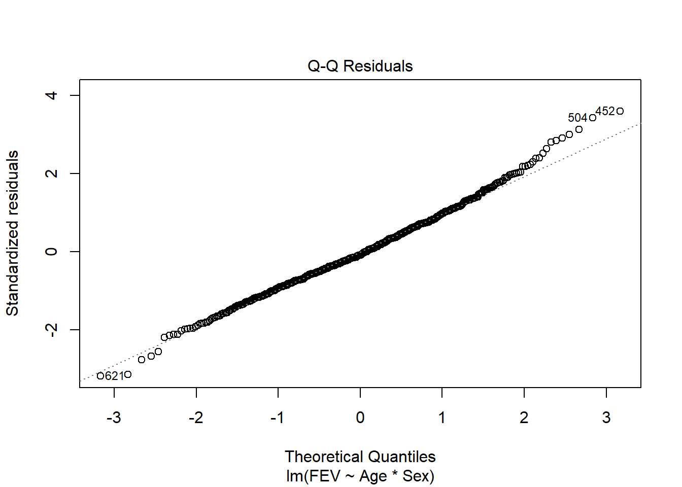
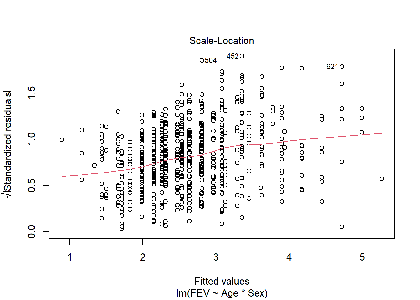
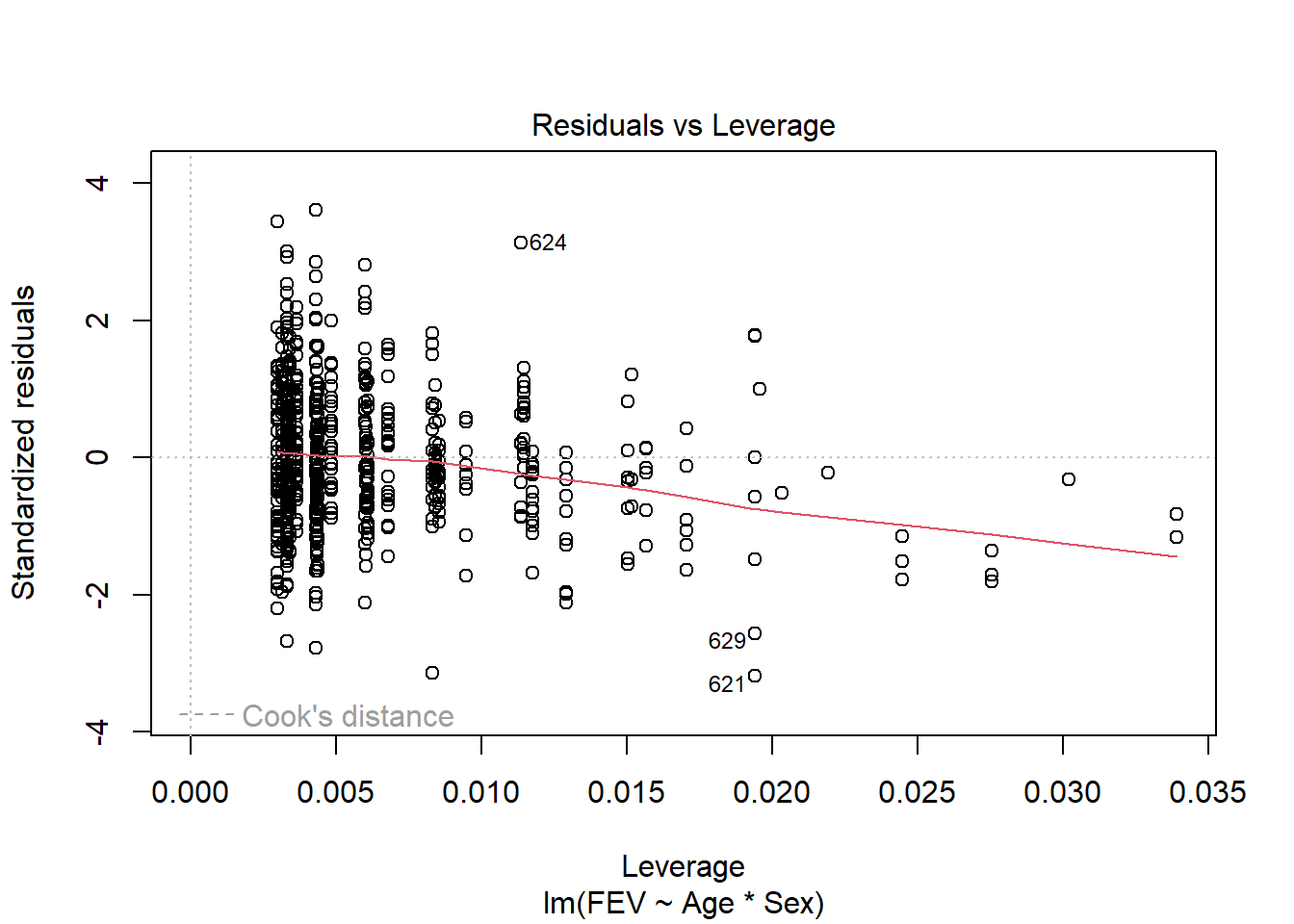
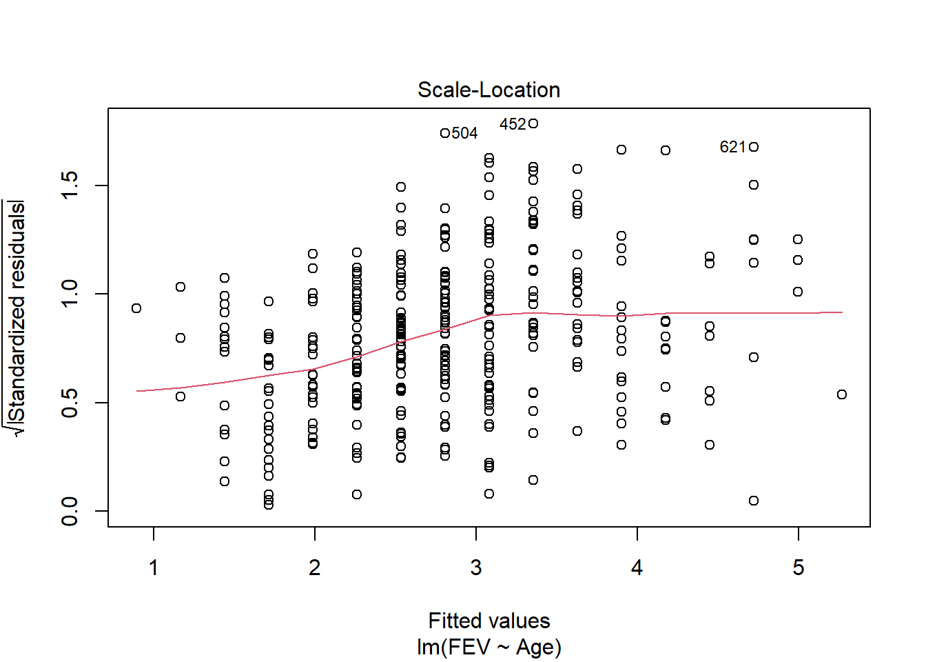
fev_age <- lm(FEV ~ Age*Sex, fev)
plot(fev_age)

library(car)
Anova(fev_age, type = "III")

Anova Table (Type III tests)

Response: FEV
             Sum Sq  Df F value    Pr(>F)    
(Intercept)  18.654   1  69.087 5.506e-16 ***
Age          72.190   1 267.356 < 2.2e-16 ***
Sex           7.977   1  29.543 7.745e-08 ***
Age:Sex      17.426   1  64.535 4.467e-15 ***
Residuals   175.509 650                      
---
Signif. codes:  0 '***' 0.001 '**' 0.01 '*' 0.05 '.' 0.1 ' ' 1

summary(fev_age)

Call:
lm(formula = FEV ~ Age * Sex, data = fev)

Residuals:
     Min       1Q   Median       3Q      Max 
-1.64072 -0.34337 -0.04934  0.33206  1.86867 

Coefficients:
             Estimate Std. Error t value Pr(>|t|)    
(Intercept)  0.849467   0.102199   8.312 5.51e-16 ***
Age          0.162729   0.009952  16.351  < 2e-16 ***
SexMale     -0.775867   0.142745  -5.435 7.74e-08 ***
Age:SexMale  0.110749   0.013786   8.033 4.47e-15 ***
---
Signif. codes:  0 '***' 0.001 '**' 0.01 '*' 0.05 '.' 0.1 ' ' 1

Residual standard error: 0.5196 on 650 degrees of freedom
Multiple R-squared:  0.6425,    Adjusted R-squared:  0.6408 
F-statistic: 389.4 on 3 and 650 DF,  p-value: < 2.2e-16

We can explore this question using an ANCOVA since the response is continuous and the explanatory variables combine a categorical and continuous variable. Analysis of residuals indicates the assumptions are met (no pattern, normal distribution). There is a significant interaction among age and gender on FEV (F_1,650=64.535, p<.001). We should explore impacts of age on each gender separately.

fev_age <- lm(FEV ~ Age, fev[fev$Sex == "Male",])
plot(fev_age)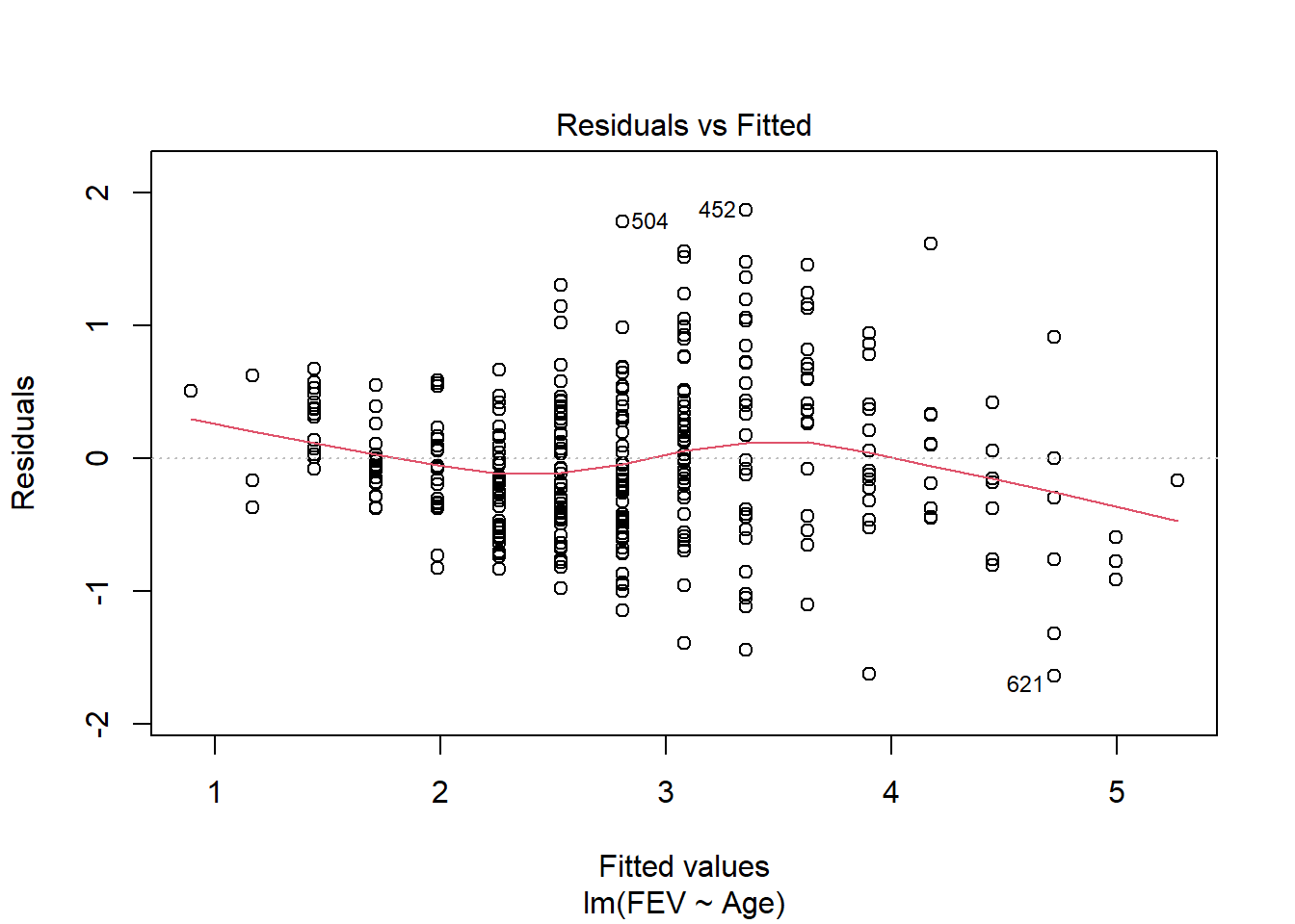

Anova(fev_age, type = "III")

Anova Table (Type III tests)

Response: FEV
             Sum Sq  Df  F value Pr(>F)    
(Intercept)   0.147   1   0.4258 0.5145    
Age         221.896   1 641.5722 <2e-16 ***
Residuals   115.518 334                    
---
Signif. codes:  0 '***' 0.001 '**' 0.01 '*' 0.05 '.' 0.1 ' ' 1

summary(fev_age)

Call:
lm(formula = FEV ~ Age, data = fev[fev$Sex == "Male", ])

Residuals:
     Min       1Q   Median       3Q      Max 
-1.64072 -0.37752 -0.05318  0.36893  1.86867 

Coefficients:
            Estimate Std. Error t value Pr(>|t|)    
(Intercept)   0.0736     0.1128   0.653    0.514    
Age           0.2735     0.0108  25.329   <2e-16 ***
---
Signif. codes:  0 '***' 0.001 '**' 0.01 '*' 0.05 '.' 0.1 ' ' 1

Residual standard error: 0.5881 on 334 degrees of freedom
Multiple R-squared:  0.6576,    Adjusted R-squared:  0.6566 
F-statistic: 641.6 on 1 and 334 DF,  p-value: < 2.2e-16

Age has a significant (F_1,334 = 641, p < 0.01) positive (.27 L yr^-1) impact on FEV in males.

fev_age <- lm(FEV ~ Age, fev[fev$Sex == "Female",])
plot(fev_age)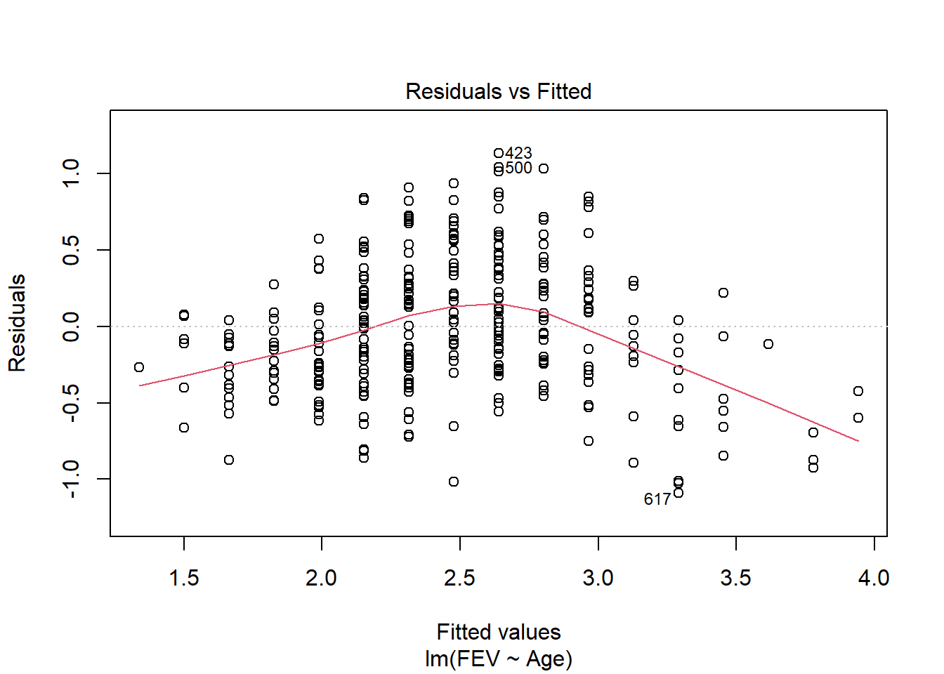

Anova(fev_age, type = "III")

Anova Table (Type III tests)

Response: FEV
            Sum Sq  Df F value    Pr(>F)    
(Intercept) 18.654   1  98.262 < 2.2e-16 ***
Age         72.190   1 380.258 < 2.2e-16 ***
Residuals   59.991 316                      
---
Signif. codes:  0 '***' 0.001 '**' 0.01 '*' 0.05 '.' 0.1 ' ' 1

summary(fev_age)

Call:
lm(formula = FEV ~ Age, data = fev[fev$Sex == "Female", ])

Residuals:
     Min       1Q   Median       3Q      Max 
-1.09240 -0.28991 -0.03762  0.28749  1.13451 

Coefficients:
            Estimate Std. Error t value Pr(>|t|)    
(Intercept) 0.849467   0.085695   9.913   <2e-16 ***
Age         0.162729   0.008345  19.500   <2e-16 ***
---
Signif. codes:  0 '***' 0.001 '**' 0.01 '*' 0.05 '.' 0.1 ' ' 1

Residual standard error: 0.4357 on 316 degrees of freedom
Multiple R-squared:  0.5461,    Adjusted R-squared:  0.5447 
F-statistic: 380.3 on 1 and 316 DF,  p-value: < 2.2e-16

Age also has a significant (F_1,316 = 380, p < 0.01) positive (.16 L yr^-1) impact on FEV in females. The interaction is likely due to the higher rate of increase of FEV with age in males.

library(ggplot2)
ggplot(fev, aes(x=Age, y=FEV, color = Sex, shape = Sex)) +
  geom_point(size = 3) +
  ylab("FEV (L)") +
  ggtitle("FEV increases faster \n with age in males")+
  theme(axis.title.x = element_text(face="bold", size=28), 
        axis.title.y = element_text(face="bold", size=28), 
        axis.text.y  = element_text(size=20),
        axis.text.x  = element_text(size=20), 
        legend.text =element_text(size=20),
        legend.title = element_text(size=20, face="bold"),
        plot.title = element_text(hjust = 0.5, face="bold", size=32)) +
    geom_smooth(method = "lm", se = F)

`geom_smooth()` using formula = 'y ~ x'

2

Data on home gas consumption at various temperatures before and after new insulation was installed has been collected @

http://www.statsci.org/data/general/insulgas.txt

More information on the data is available @

http://www.statsci.org/data/general/insulgas.html

Is there any relationship between these factors? How would you test this, and what type of plot would you produce to accompany your analysis?

heat <- read.table("http://www.statsci.org/data/general/insulgas.txt", 
                   header = T, stringsAsFactors = T)
head(heat)

  Insulate Temp Gas
1   Before -0.8 7.2
2   Before -0.7 6.9
3   Before  0.4 6.4
4   Before  2.5 6.0
5   Before  2.9 5.8
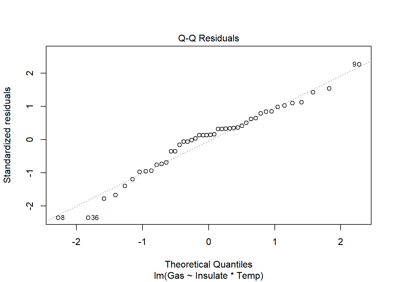
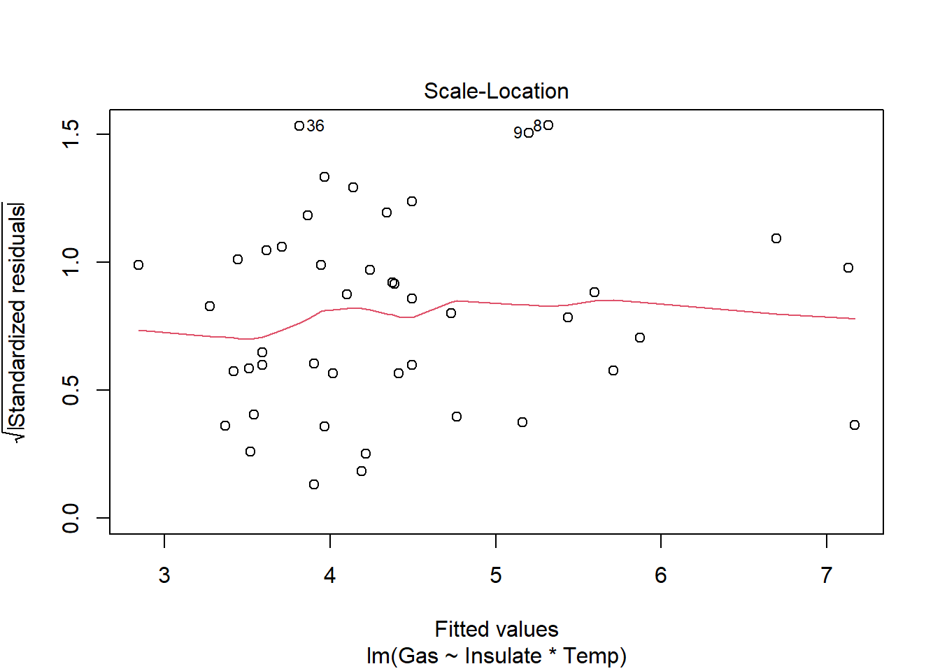
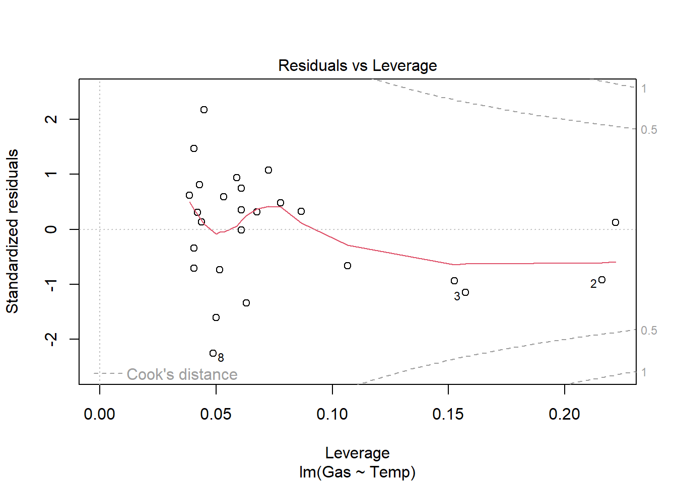
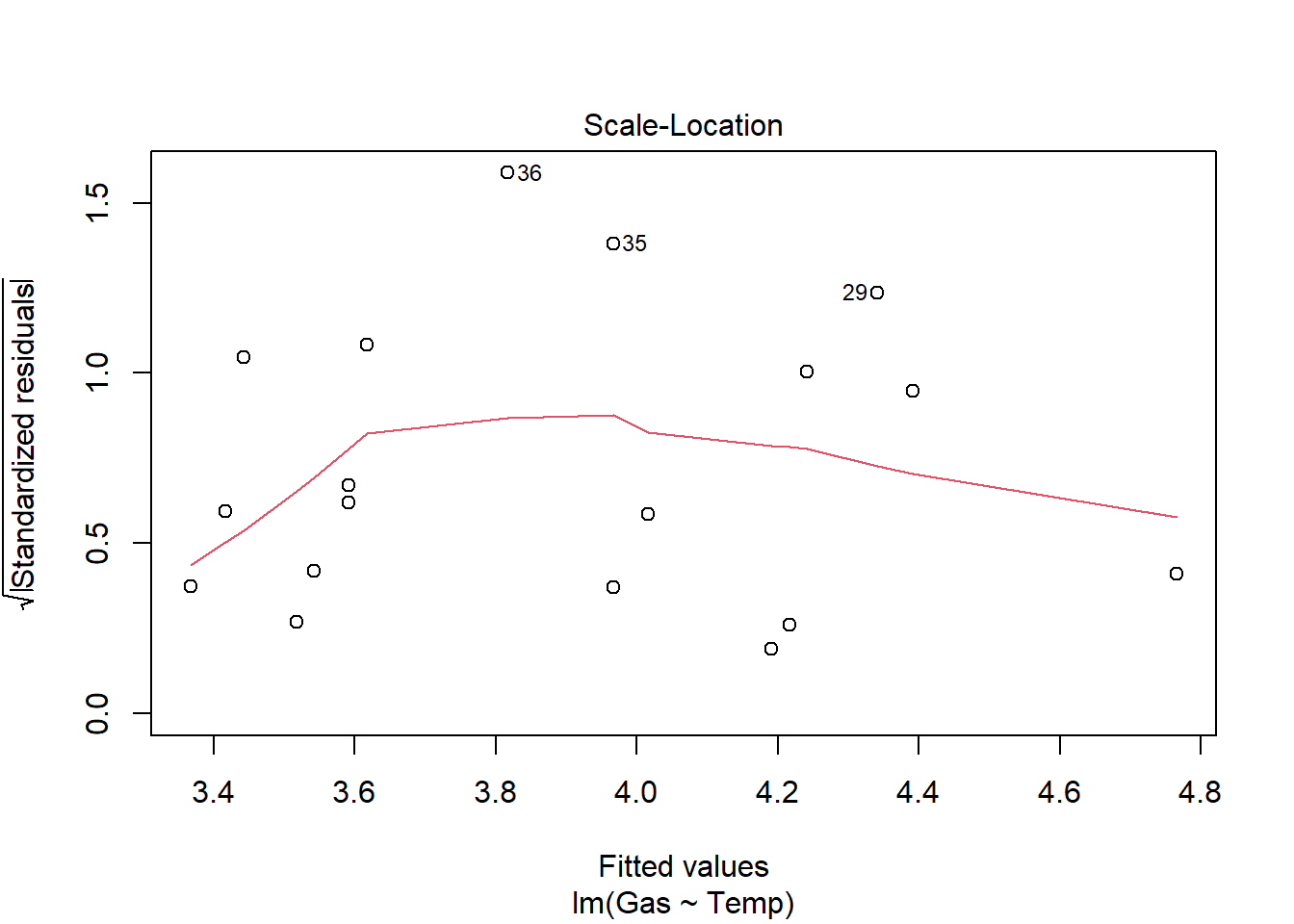
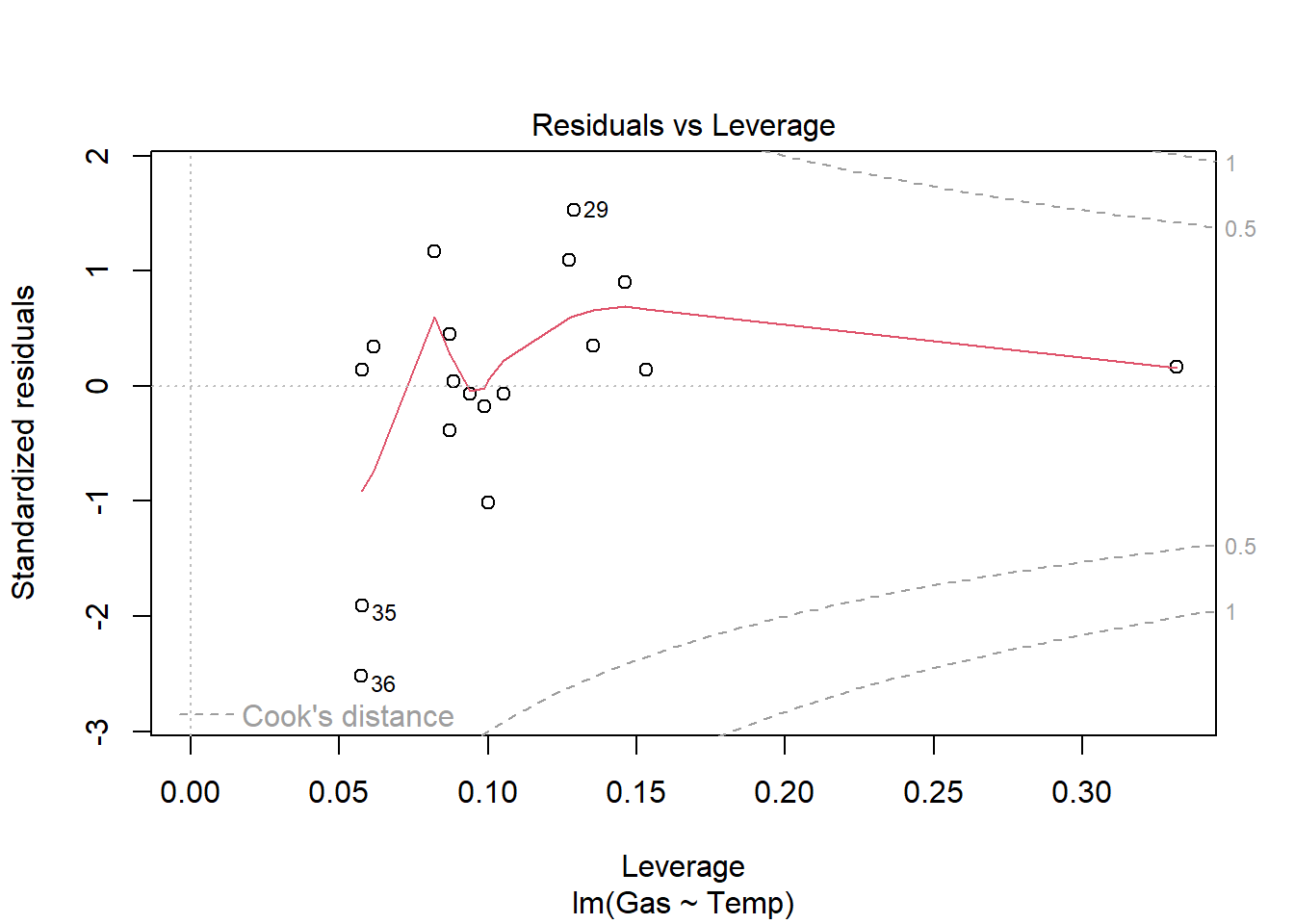
6   Before  3.2 5.8

heat_model <- lm(Gas ~ Insulate * Temp, heat)
plot(heat_model)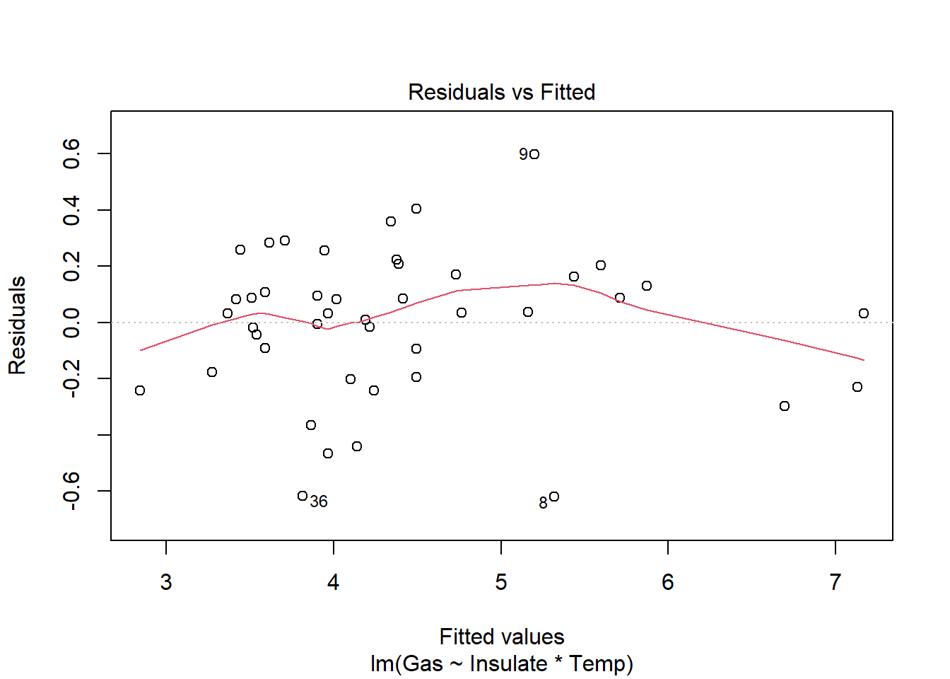

require(car)
Anova(heat_model, type = "III")

Anova Table (Type III tests)

Response: Gas
              Sum Sq Df  F value    Pr(>F)    
(Intercept)   90.636  1 1243.911 < 2.2e-16 ***
Insulate      12.502  1  171.583 4.709e-16 ***
Temp           2.783  1   38.191 2.640e-07 ***
Insulate:Temp  0.757  1   10.391  0.002521 ** 
Residuals      2.915 40                       
---
Signif. codes:  0 '***' 0.001 '**' 0.01 '*' 0.05 '.' 0.1 ' ' 1

ggplot(heat, aes_string(x="Temp", y="Gas", color = "Insulate")) +
  geom_point(size = 3) +
  ylab(expression(paste("Gas (1000 ",ft^3, ")")))+
  xlab(expression(paste("Temperature (", degree~C, ")")))+
  geom_smooth(method = "lm", se = F) +
  theme(axis.title.x = element_text(face="bold", size=28), 
        axis.title.y = element_text(face="bold", size=28), 
        axis.text.y  = element_text(size=20),
        axis.text.x  = element_text(size=20), 
        legend.text =element_text(size=20),
        legend.title = element_text(size=20, face="bold"),
        plot.title = element_text(hjust = 0.5, face="bold", size=32))

Warning: `aes_string()` was deprecated in ggplot2 3.0.0.
ℹ Please use tidy evaluation idioms with `aes()`.
ℹ See also `vignette("ggplot2-in-packages")` for more information.

`geom_smooth()` using formula = 'y ~ x'

There is a significant relationship between insulation type (before/after) and temperature on gas usage (F_1,40=10.39, p<.01). Graphical analysis indicates the old (before) insulation led to higher overall gas usage and gas usage increased faster with colder temperature compared to the new insulation. Statistical analysis bears this out

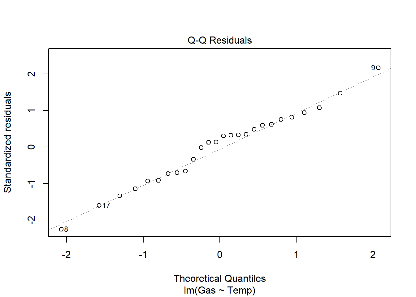
heat_model_old <- lm(Gas ~ Temp, heat[heat$Insulate == "Before",])
plot(heat_model_old)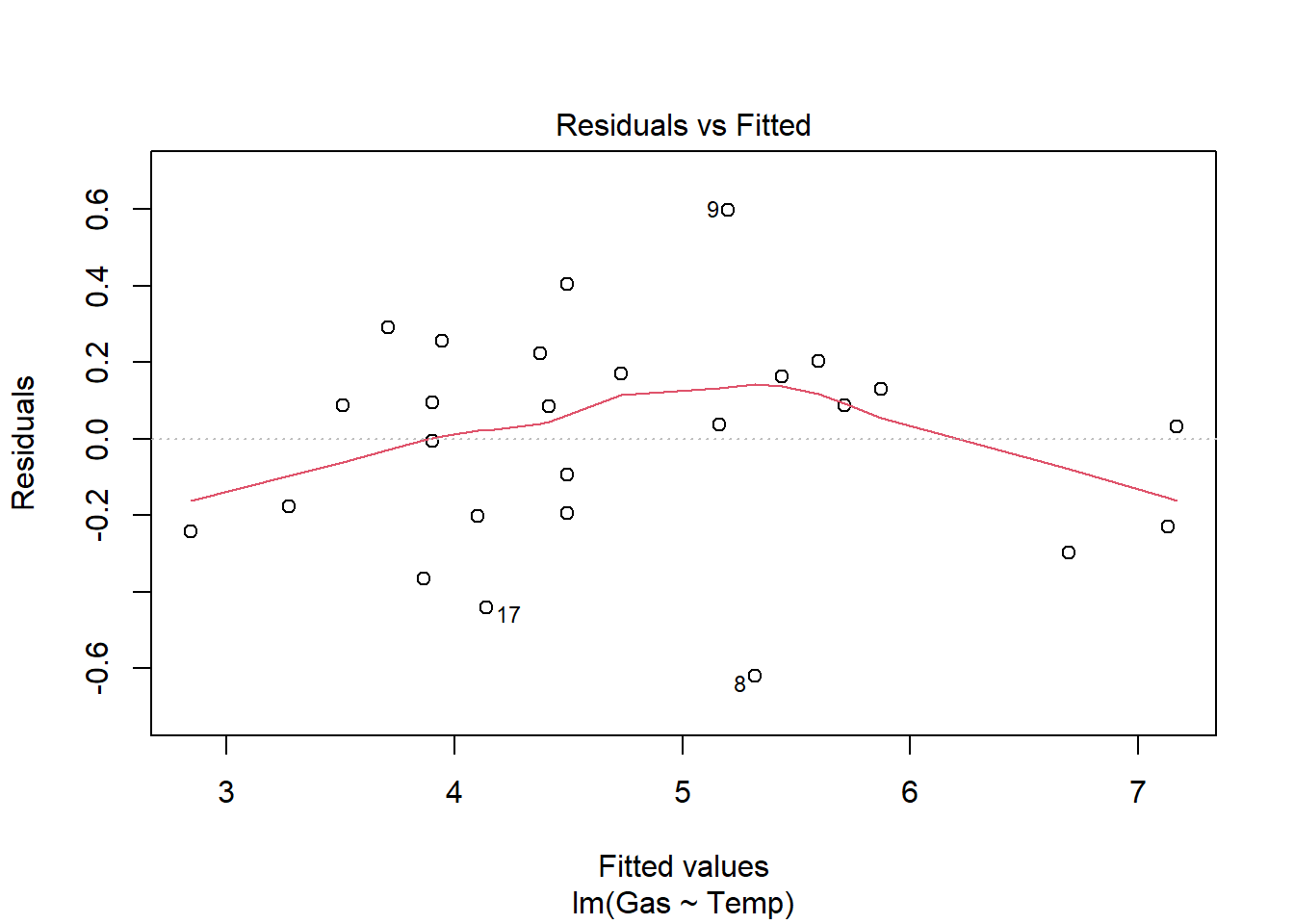

summary(heat_model_old)

Call:
lm(formula = Gas ~ Temp, data = heat[heat$Insulate == "Before", 
    ])

Residuals:
     Min       1Q   Median       3Q      Max 
-0.62020 -0.19947  0.06068  0.16770  0.59778 

Coefficients:
            Estimate Std. Error t value Pr(>|t|)    
(Intercept)  6.85383    0.11842   57.88   <2e-16 ***
Temp        -0.39324    0.01959  -20.08   <2e-16 ***
---
Signif. codes:  0 '***' 0.001 '**' 0.01 '*' 0.05 '.' 0.1 ' ' 1

Residual standard error: 0.2813 on 24 degrees of freedom
Multiple R-squared:  0.9438,    Adjusted R-squared:  0.9415 
F-statistic: 403.1 on 1 and 24 DF,  p-value: < 2.2e-16

Anova(heat_model_old, type = "III")

Anova Table (Type III tests)

Response: Gas
             Sum Sq Df F value    Pr(>F)    
(Intercept) 265.115  1 3349.59 < 2.2e-16 ***
Temp         31.905  1  403.11 < 2.2e-16 ***
Residuals     1.900 24                      
---
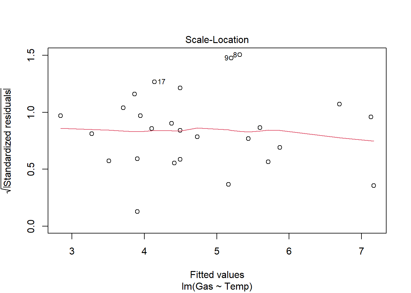
Signif. codes:  0 '***' 0.001 '**' 0.01 '*' 0.05 '.' 0.1 ' ' 1

heat_model_new<- lm(Gas ~ Temp, heat[heat$Insulate == "After",])
plot(heat_model_new)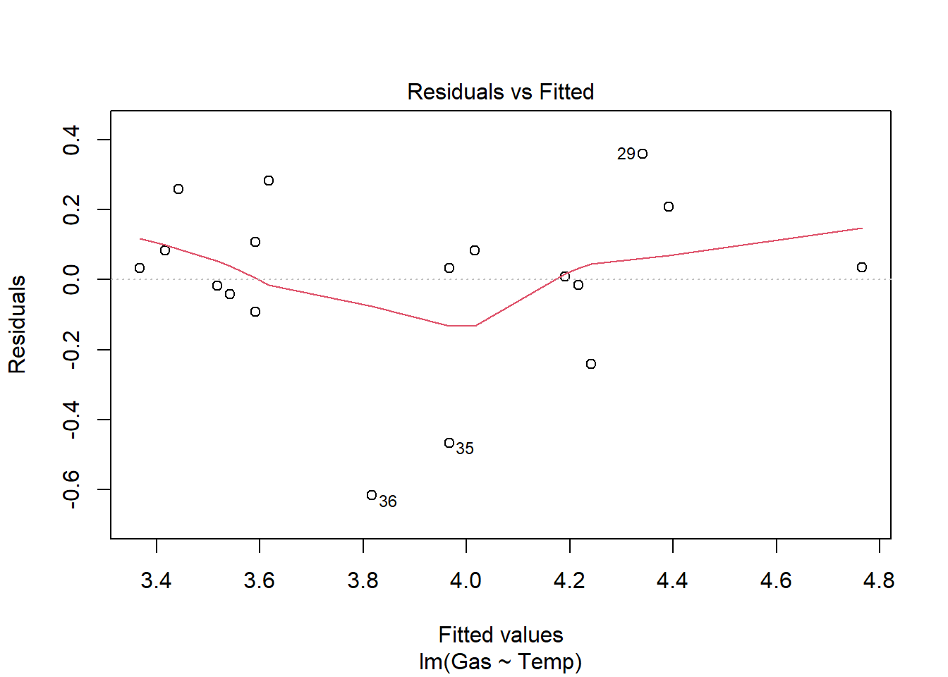

summary(heat_model_new)

Call:
lm(formula = Gas ~ Temp, data = heat[heat$Insulate == "After", 
    ])

Residuals:
     Min       1Q   Median       3Q      Max 
-0.61677 -0.03594  0.03300  0.10180  0.35901 

Coefficients:
            Estimate Std. Error t value Pr(>|t|)    
(Intercept)  4.59062    0.12145  37.799  < 2e-16 ***
Temp        -0.24963    0.03769  -6.623 5.86e-06 ***
---
Signif. codes:  0 '***' 0.001 '**' 0.01 '*' 0.05 '.' 0.1 ' ' 1

Residual standard error: 0.2519 on 16 degrees of freedom
Multiple R-squared:  0.7327,    Adjusted R-squared:  0.716 
F-statistic: 43.87 on 1 and 16 DF,  p-value: 5.857e-06

Anova(heat_model_new, type = "III")

Anova Table (Type III tests)

Response: Gas
            Sum Sq Df  F value    Pr(>F)    
(Intercept) 90.636  1 1428.759 < 2.2e-16 ***
Temp         2.783  1   43.867 5.857e-06 ***
Residuals    1.015 16                       
---
Signif. codes:  0 '***' 0.001 '**' 0.01 '*' 0.05 '.' 0.1 ' ' 1

There is a significant relationship between gas usage and temperature for old and new insulation homes. However, the old insulation led to using 400 ft³ more gas per week to heat the house with every degree drop in temperature, while the new insulation leads to a increase of only 250 ft³ more gas per week with each degree drop.

3

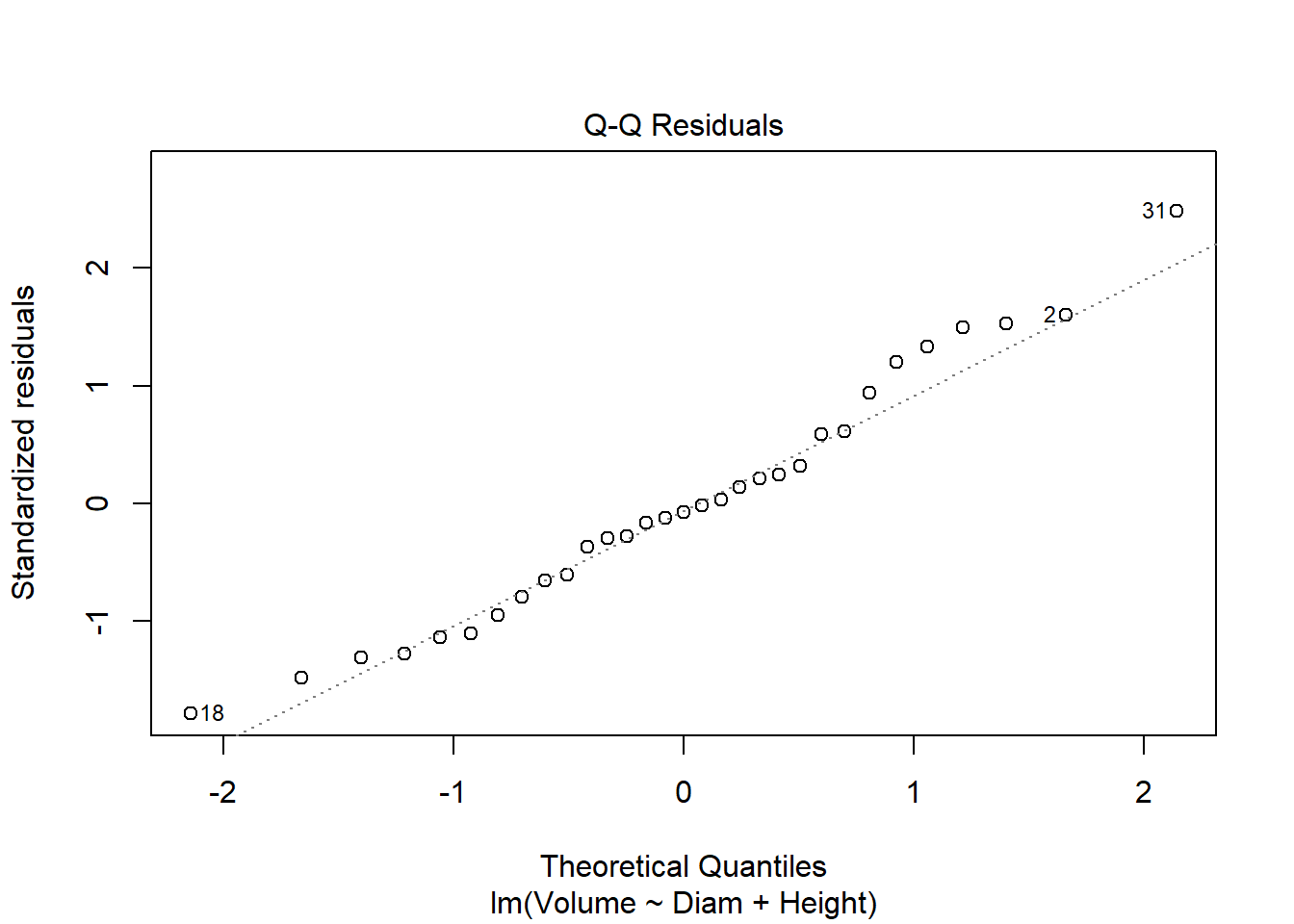
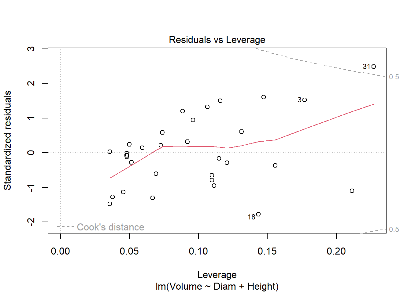
Data on the height, diameter, and volume of cherry trees was collected for use in developing an optimal model to predict timber volume. Data is available @

http://www.statsci.org/data/general/cherry.txt

Use the data to justify an optimal model.

cherry <- read.table("http://www.statsci.org/data/general/cherry.txt",
                     header = T)
head(cherry)

  Diam Height Volume
1  8.3     70   10.3
2  8.6     65   10.3
3  8.8     63   10.2
4 10.5     72   16.4
5 10.7     81   18.8
6 10.8     83   19.7

#if only considering main effects (one option)
cherry_full <- lm(Volume ~ Diam + Height, cherry)
plot(cherry_full)

library(car)
Anova(cherry_full, type = "III")

Anova Table (Type III tests)

Response: Volume
            Sum Sq Df  F value    Pr(>F)    
(Intercept)  679.0  1  45.0632  2.75e-07 ***
Diam        4783.0  1 317.4129 < 2.2e-16 ***
Height       102.4  1   6.7943   0.01449 *  
Residuals    421.9 28                       
---
Signif. codes:  0 '***' 0.001 '**' 0.01 '*' 0.05 '.' 0.1 ' ' 1

#both are significant, so finished

#could also consider interactions 
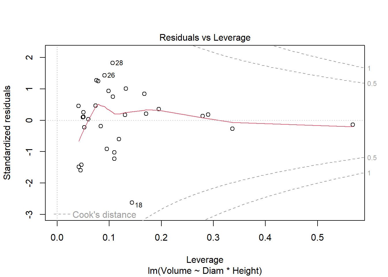
cherry_full <- lm(Volume ~ Diam * Height, cherry)
plot(cherry_full)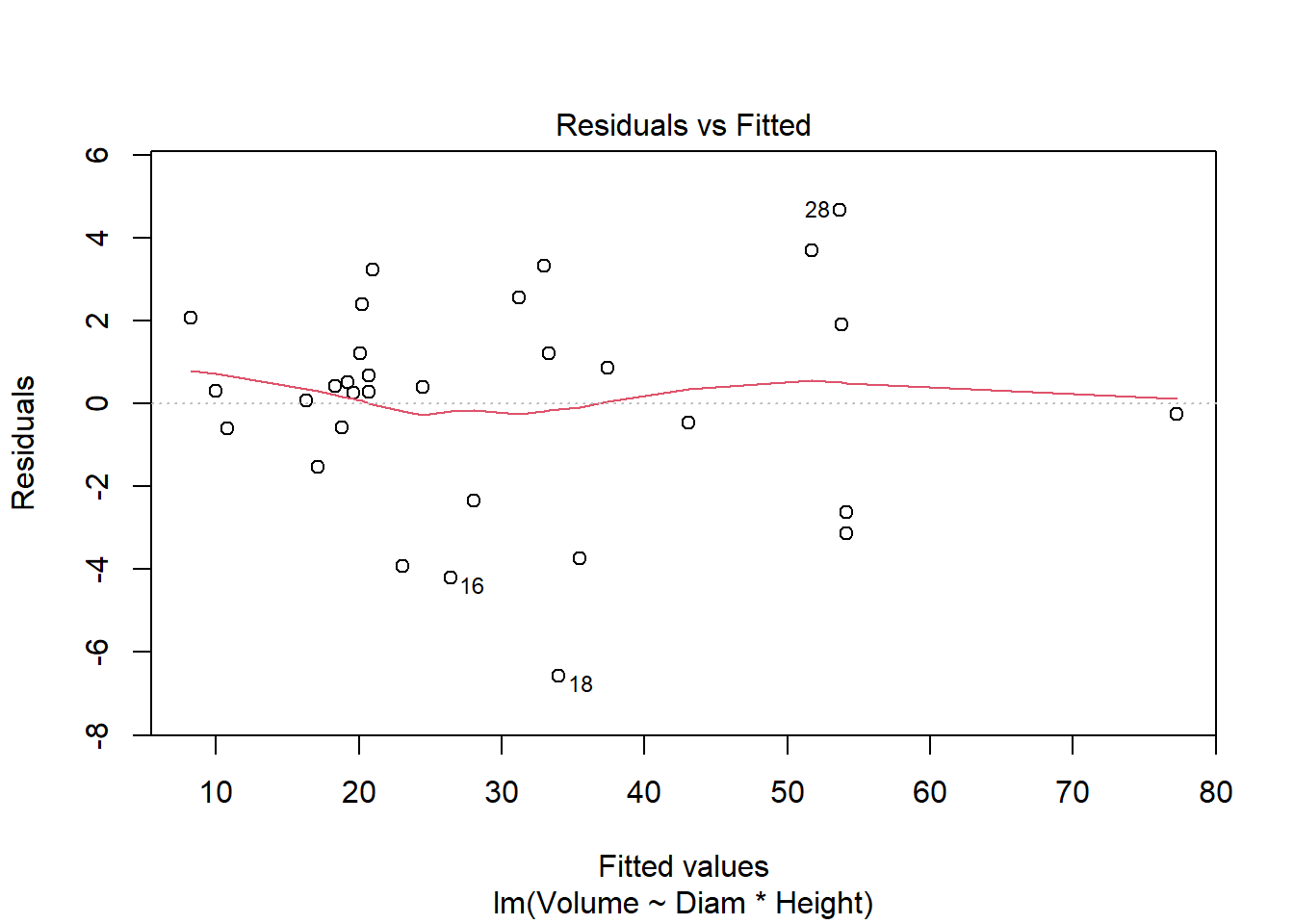

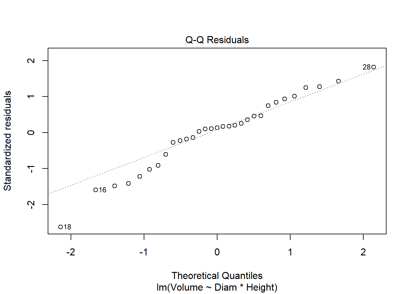
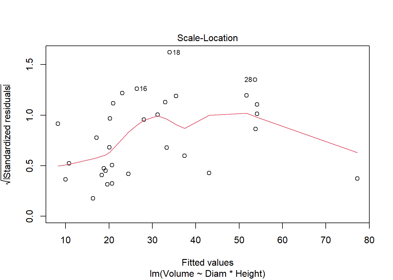
Anova(cherry_full, type = "III")

Anova Table (Type III tests)

Response: Volume
             Sum Sq Df F value    Pr(>F)    
(Intercept)  62.185  1  8.4765 0.0071307 ** 
Diam         68.147  1  9.2891 0.0051087 ** 
Height      128.566  1 17.5248 0.0002699 ***
Diam:Height 223.843  1 30.5119 7.484e-06 ***
Residuals   198.079 27                      
---
Signif. codes:  0 '***' 0.001 '**' 0.01 '*' 0.05 '.' 0.1 ' ' 1

summary(cherry_full)

Call:
lm(formula = Volume ~ Diam * Height, data = cherry)

Residuals:
    Min      1Q  Median      3Q     Max 
-6.5821 -1.0673  0.3026  1.5641  4.6649 

Coefficients:
            Estimate Std. Error t value Pr(>|t|)    
(Intercept) 69.39632   23.83575   2.911  0.00713 ** 
Diam        -5.85585    1.92134  -3.048  0.00511 ** 
Height      -1.29708    0.30984  -4.186  0.00027 ***
Diam:Height  0.13465    0.02438   5.524 7.48e-06 ***
---
Signif. codes:  0 '***' 0.001 '**' 0.01 '*' 0.05 '.' 0.1 ' ' 1

Residual standard error: 2.709 on 27 degrees of freedom
Multiple R-squared:  0.9756,    Adjusted R-squared:  0.9728 
F-statistic: 359.3 on 3 and 27 DF,  p-value: < 2.2e-16

#all significant, so finished

I used multiple regression to consider the impacts of both continuous and categorical explanatory variables on timber volume. I used a top-down approach focused on p-values (F tests) in this example. Both diameter and height (and their interaction) are significant, so the full model is justified by the data. It explains 97.5% of the variation in volume. AIC methods lead to a similar outcome

library(MASS)
stepAIC(cherry_full)

Start:  AIC=65.49
Volume ~ Diam * Height

              Df Sum of Sq    RSS    AIC
<none>                     198.08 65.495
- Diam:Height  1    223.84 421.92 86.936

Call:
lm(formula = Volume ~ Diam * Height, data = cherry)

Coefficients:
(Intercept)         Diam       Height  Diam:Height  
    69.3963      -5.8558      -1.2971       0.1347  

4

Over the course of five years, a professor asked students in his stats class to carry out a simple experiment. Students were asked to measure their pulse rate, run for one minute, then measure their pulse rate again. The students also filled out a questionnaire. Data include:

Variable	Description
Height	Height (cm)
Weight	Weight (kg)
Age	Age (years)
Gender	Sex (1 = male, 2 = female)
Smokes	Regular smoker? (1 = yes, 2 = no)
Alcohol	Regular drinker? (1 = yes, 2 = no)
Exercise	Frequency of exercise (1 = high, 2 = moderate, 3 = low)
Change	Percent change in pulse (pulse after experiment/pulse before experiment)
Year	Year of class (93 - 98)

Using the available data (available at

https://docs.google.com/spreadsheets/d/e/2PACX-1vToN77M80enimQglwpFroooLzDtcQMh4qKbOuhbu-eVmU9buczh7nVV1BdI4T_ma-PfWUnQYmq-60RZ/pub?gid=942311716&single=true&output=csv )

determine the optimal subset of explanatory variables that should be used to predict change pulse rate (Change) (focusing on main effects only, no interactions) and explain your choice of methods. Interpret your results. Make sure you can explain any changes you needed to make to the dataset or steps you used in your analysis.

pulse_class_copy <- read.csv("https://docs.google.com/spreadsheets/d/e/2PACX-1vToN77M80enimQglwpFroooLzDtcQMh4qKbOuhbu-eVmU9buczh7nVV1BdI4T_ma-PfWUnQYmq-60RZ/pub?gid=942311716&single=true&output=csv", stringsAsFactors = T)
pulse_class_copy$Gender <- as.factor(pulse_class_copy$Gender)
pulse_class_copy$Smokes <- as.factor (pulse_class_copy$Smokes)
pulse_class_copy$Alcohol <- as.factor(pulse_class_copy$Alcohol)

pulse_full <- lm(Change ~ ., pulse_class_copy )
pulse_final <- step(pulse_full)

Start:  AIC=-94.24
Change ~ Height + Weight + Age + Gender + Smokes + Alcohol + 
    Exercise + Year

           Df Sum of Sq    RSS     AIC
- Year      1  0.002178 4.0113 -96.218
- Gender    1  0.002825 4.0119 -96.211
- Smokes    1  0.006969 4.0161 -96.163
- Age       1  0.007498 4.0166 -96.157
- Weight    1  0.018975 4.0281 -96.026
- Exercise  1  0.063201 4.0723 -95.524
<none>                  4.0091 -94.243
- Height    1  0.248912 4.2580 -93.473
- Alcohol   1  0.275592 4.2847 -93.185

Step:  AIC=-96.22
Change ~ Height + Weight + Age + Gender + Smokes + Alcohol + 
    Exercise

           Df Sum of Sq    RSS     AIC
- Gender    1  0.002745 4.0140 -98.187
- Smokes    1  0.008748 4.0200 -98.118
- Age       1  0.009061 4.0203 -98.115
- Weight    1  0.020656 4.0319 -97.982
- Exercise  1  0.061106 4.0724 -97.523
<none>                  4.0113 -96.218
- Height    1  0.247630 4.2589 -95.463
- Alcohol   1  0.280615 4.2919 -95.108

Step:  AIC=-98.19
Change ~ Height + Weight + Age + Smokes + Alcohol + Exercise

           Df Sum of Sq    RSS      AIC
- Age       1  0.008872 4.0229 -100.085
- Smokes    1  0.009773 4.0238 -100.075
- Weight    1  0.019557 4.0336  -99.963
- Exercise  1  0.058622 4.0726  -99.520
<none>                  4.0140  -98.187
- Height    1  0.258061 4.2721  -97.321
- Alcohol   1  0.302450 4.3165  -96.845

Step:  AIC=-100.09
Change ~ Height + Weight + Smokes + Alcohol + Exercise

           Df Sum of Sq    RSS      AIC
- Smokes    1  0.009335 4.0322 -101.979
- Weight    1  0.020707 4.0436 -101.849
- Exercise  1  0.063527 4.0864 -101.365
<none>                  4.0229 -100.085
- Height    1  0.270131 4.2930  -99.096
- Alcohol   1  0.293626 4.3165  -98.845

Step:  AIC=-101.98
Change ~ Height + Weight + Alcohol + Exercise

           Df Sum of Sq    RSS     AIC
- Weight    1  0.020452 4.0527 -103.75
- Exercise  1  0.055663 4.0879 -103.35
<none>                  4.0322 -101.98
- Height    1  0.263914 4.2961 -101.06
- Alcohol   1  0.285822 4.3181 -100.83

Step:  AIC=-103.75
Change ~ Height + Alcohol + Exercise

           Df Sum of Sq    RSS     AIC
- Exercise  1   0.07307 4.1258 -104.92
<none>                  4.0527 -103.75
- Alcohol   1   0.28662 4.3393 -102.60
- Height    1   0.39237 4.4451 -101.50

Step:  AIC=-104.92
Change ~ Height + Alcohol

          Df Sum of Sq    RSS     AIC
<none>                 4.1258 -104.92
- Alcohol  1   0.25346 4.3792 -104.18
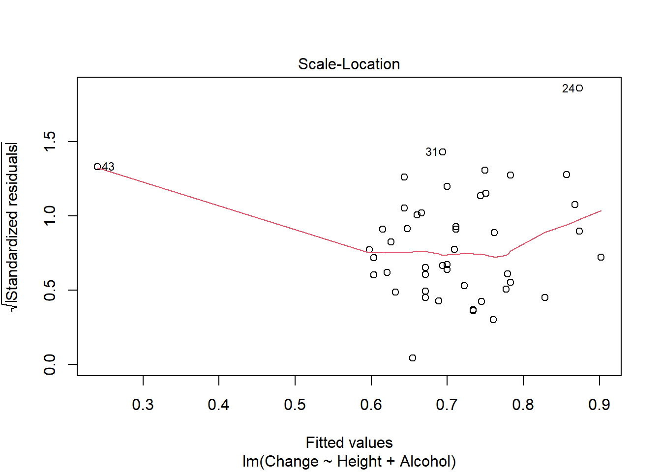
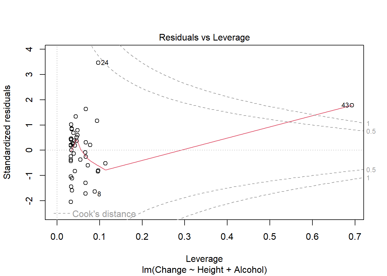
- Height   1   0.43164 4.5574 -102.35

#consider assumptions
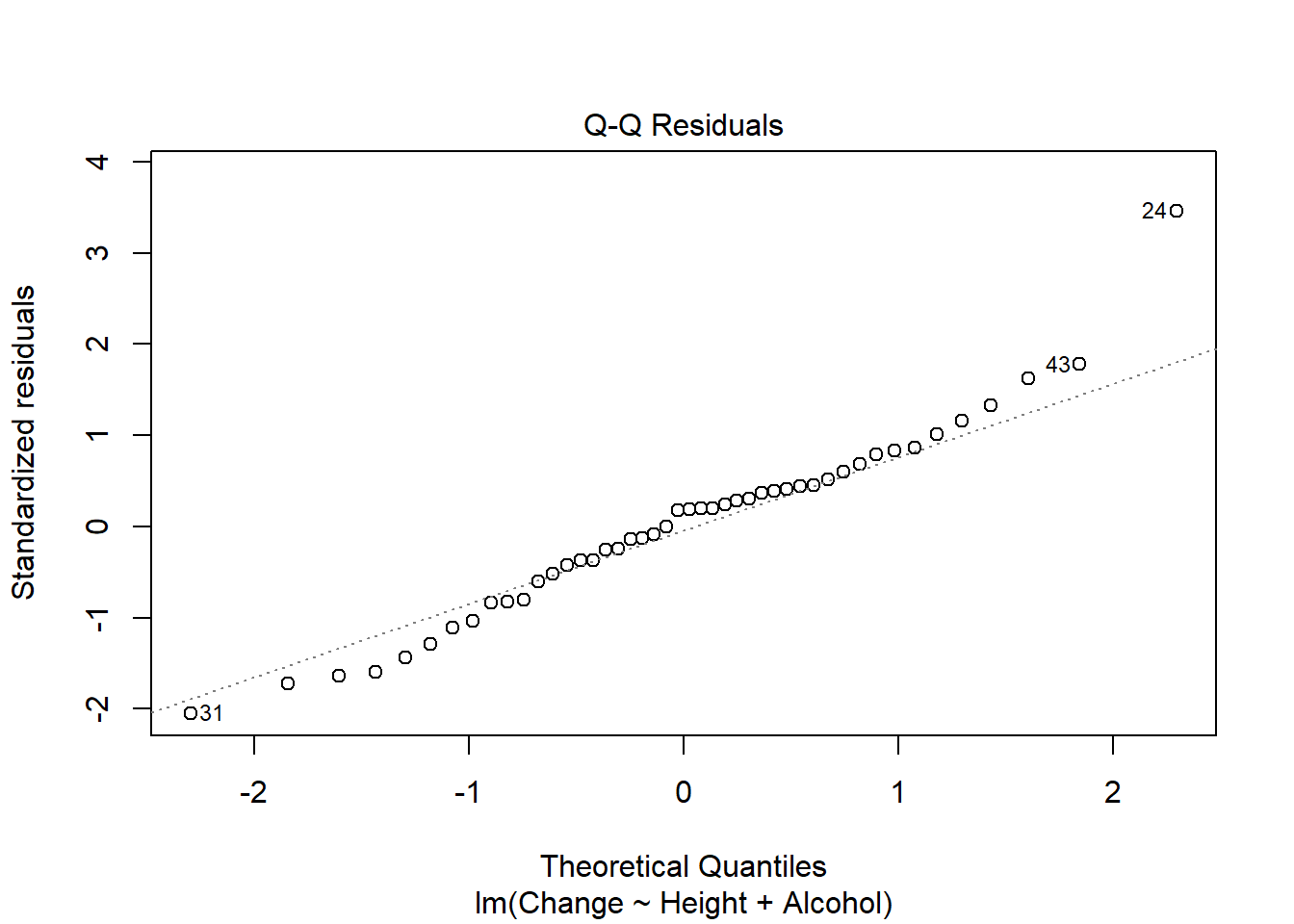
plot(pulse_final)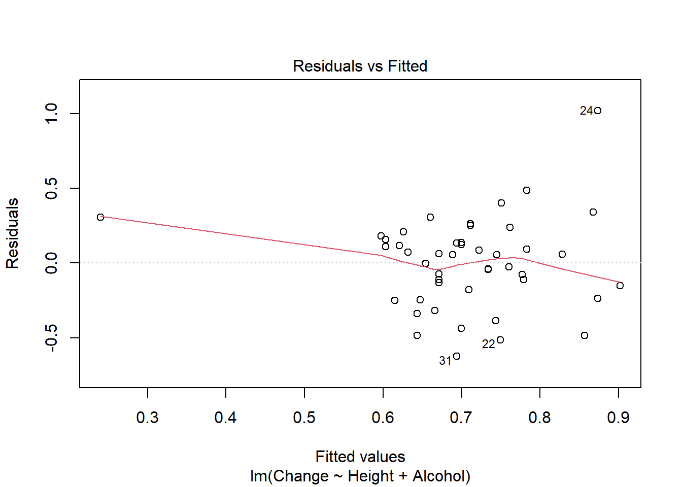

Anova(pulse_final, type = "III")

Anova Table (Type III tests)

Response: Change
            Sum Sq Df F value  Pr(>F)  
(Intercept) 0.0434  1  0.4520 0.50500  
Height      0.4316  1  4.4987 0.03973 *
Alcohol     0.2535  1  2.6416 0.11141  
Residuals   4.1258 43                  
---
Signif. codes:  0 '***' 0.001 '**' 0.01 '*' 0.05 '.' 0.1 ' ' 1

summary(pulse_final)

Call:
lm(formula = Change ~ Height + Alcohol, data = pulse_class_copy)

Residuals:
     Min       1Q   Median       3Q      Max 
-0.62511 -0.17315  0.05539  0.15239  1.01992 

Coefficients:
             Estimate Std. Error t value Pr(>|t|)  
(Intercept) -0.318699   0.474060  -0.672   0.5050  
Height       0.005658   0.002668   2.121   0.0397 *
Alcohol2     0.173965   0.107035   1.625   0.1114  
---
Signif. codes:  0 '***' 0.001 '**' 0.01 '*' 0.05 '.' 0.1 ' ' 1

Residual standard error: 0.3098 on 43 degrees of freedom
Multiple R-squared:  0.1074,    Adjusted R-squared:  0.06585 
F-statistic: 2.586 on 2 and 43 DF,  p-value: 0.08699

#or
library(MuMIn)
options(na.action = "na.fail")
auto <- dredge(pulse_full)

Fixed term is "(Intercept)"

library(rmarkdown)
paged_table(auto)

options(na.action = "na.omit")

I used step based approach (which requires nested models) and large search method above. Using the step approach only height and alcohol usage are retained in the final model, which explains 10% of the variation in pulse change. Model assumptions are also met. The search method finds the same optimal model but notes many other models (including a null model) perform similarly well.

5

Find one example of model selection from a paper in your field. It may be more complicated (see next question!) than what we have done, but try to identify the approach (F/AIC, top-down/bottom-up/not nested) they used. Review how they explained their approach (methods) and reported outcomes (results). Be prepared to discuss in class next week.

6

Find one example of a linear model selection (e.g., generalized linear models, mixed-effects models, beta regression) from a paper in your field. Be prepared to name the technique in class next week.