More ANOVAs

Remember you should

• add code chunks by clicking the Insert Chunk button on the toolbar or by pressing Ctrl+Alt+I to answer the questions!
• render your file to produce a markdown version that you can see!
• save your work often
  • commit it via git!
  • push updates to github

Overview

This practice reviews the More ANOVAs lecuture.

Examples

If interaction is significant

Following the memory example from class, read in and check data

memory <- read.table("http://www.statsci.org/data/general/eysenck.txt", header = T,
                     stringsAsFactors = T)
str(memory)

'data.frame':   100 obs. of  3 variables:
 $ Age    : Factor w/ 2 levels "Older","Younger": 2 2 2 2 2 2 2 2 2 2 ...
 $ Process: Factor w/ 5 levels "Adjective","Counting",..: 2 2 2 2 2 2 2 2 2 2 ...
 $ Words  : num  8 6 4 6 7 6 5 7 9 7 ...

Let’s put younger level first

library(plyr)
memory$Age <- relevel(memory$Age, "Younger")

and graph

library(Rmisc)

Warning: package 'Rmisc' was built under R version 4.3.1

Loading required package: lattice

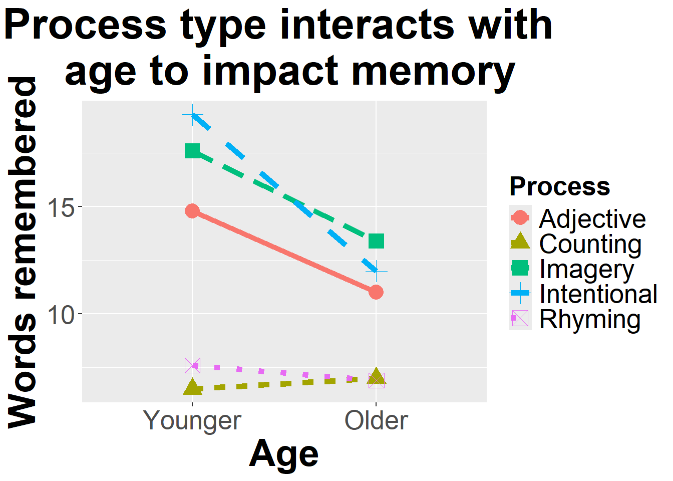
function_output <- summarySE(memory, measurevar="Words", groupvars =
                               c("Age", "Process"), na.rm = T)
library(ggplot2)

Warning: package 'ggplot2' was built under R version 4.3.3

ggplot(function_output, aes(x=Age, y=Words,color=Process, 
                                   shape = Process)) +
  geom_line(aes(group=Process, linetype = Process), size=2) +
    geom_point(size = 5) +
  ylab("Words remembered")+ 
  xlab("Age") + 
  ggtitle("Process type interacts with age to impact memory")+
  theme(axis.title.x = element_text(face="bold", size=28), 
        axis.title.y = element_text(face="bold", size=28), 
        axis.text.y  = element_text(size=20),
        axis.text.x  = element_text(size=20), 
        legend.text =element_text(size=20),
        legend.title = element_text(size=20, face="bold"),
        plot.title = element_text(hjust = 0.5, face="bold", size=32))

Warning: Using `size` aesthetic for lines was deprecated in ggplot2 3.4.0.
ℹ Please use `linewidth` instead.

There appears to be some interactions. Let’ build a model

memory_interactions <- lm(Words ~ Age * Process, memory)

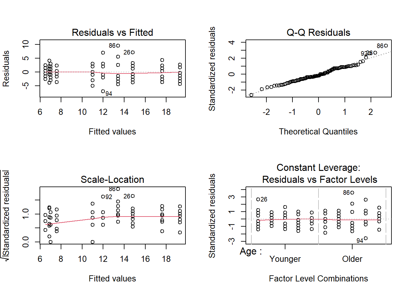
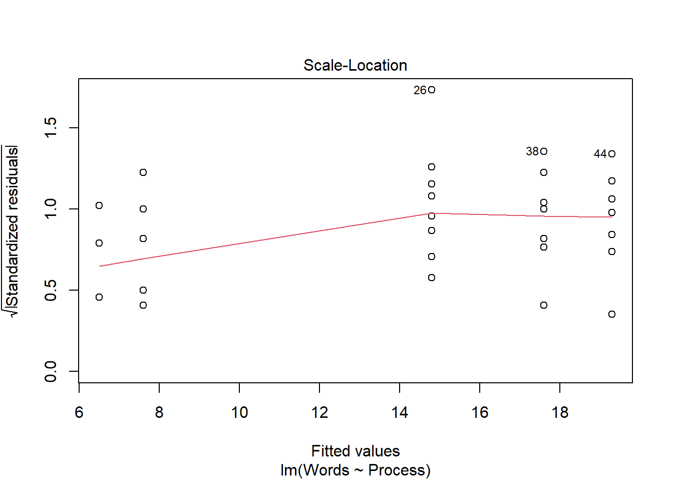
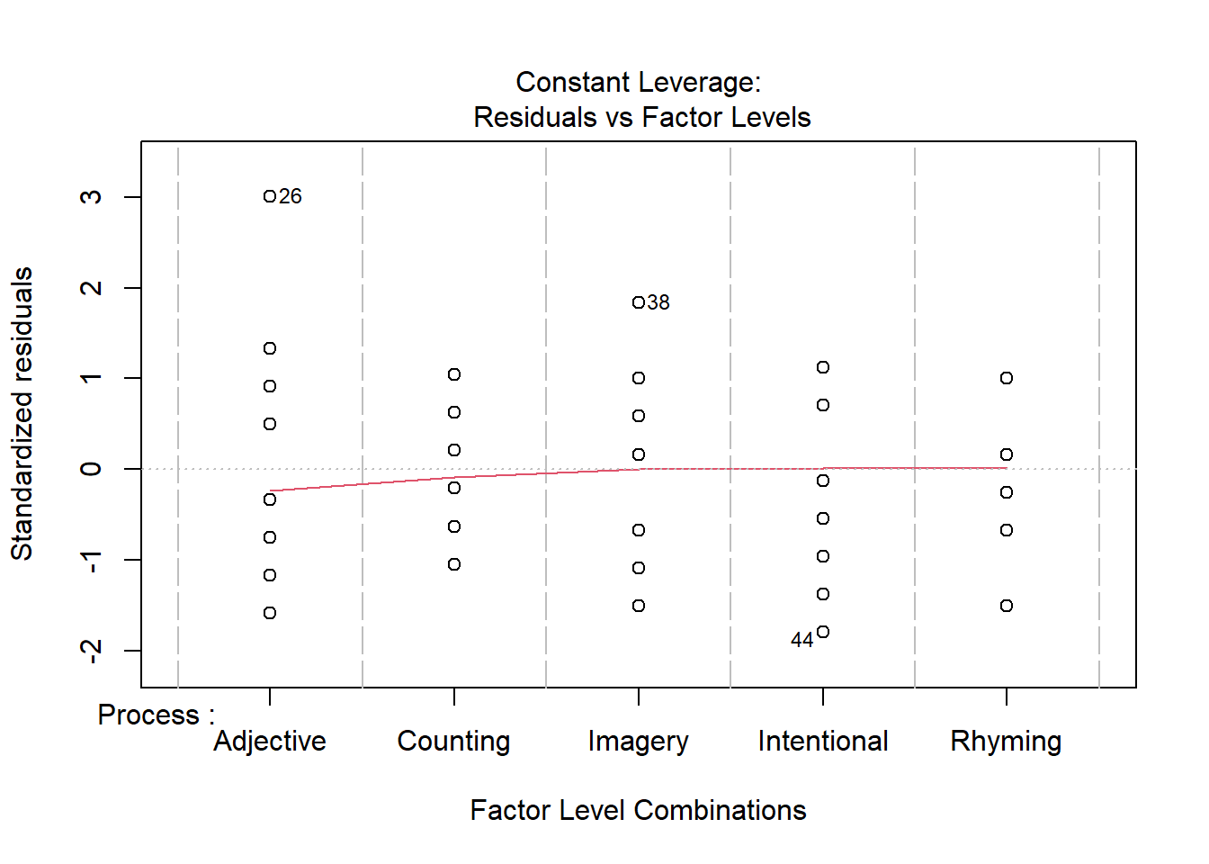
and check assumptions.

par(mfrow=c(2,2))
plot(memory_interactions)

These appear to be met, so look at output

library(car)

Warning: package 'car' was built under R version 4.3.1

Loading required package: carData

Anova(memory_interactions, type = "III")

Anova Table (Type III tests)

Response: Words
            Sum Sq Df  F value    Pr(>F)    
(Intercept) 2190.4  1 272.9281 < 2.2e-16 ***
Age           72.2  1   8.9963 0.0034984 ** 
Process     1353.7  4  42.1690 < 2.2e-16 ***
Age:Process  190.3  4   5.9279 0.0002793 ***
Residuals    722.3 90                       
---
Signif. codes:  0 '***' 0.001 '**' 0.01 '*' 0.05 '.' 0.1 ' ' 1

Since interaction is significant, analyze subsets. For example,

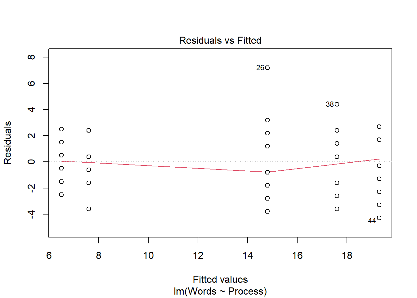
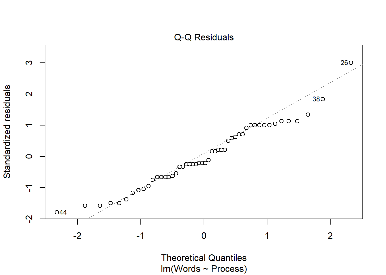
memory_interactions_young <- lm(Words ~ Process, memory[memory$Age == "Younger",])
plot(memory_interactions_young)

Anova(memory_interactions_young, type = "III")

Anova Table (Type III tests)

Response: Words
            Sum Sq Df F value    Pr(>F)    
(Intercept) 2190.4  1 343.442 < 2.2e-16 ***
Process     1353.7  4  53.064 < 2.2e-16 ***
Residuals    287.0 45                      
---
Signif. codes:  0 '***' 0.001 '**' 0.01 '*' 0.05 '.' 0.1 ' ' 1

There is a significant difference in words recalled based on process, but why? Investigate with post-hoc tests.

library(multcomp)

Loading required package: mvtnorm

Loading required package: survival

Loading required package: TH.data

Loading required package: MASS

Attaching package: 'TH.data'

The following object is masked from 'package:MASS':

    geyser

comp_young <- glht(memory_interactions_young, linfct = mcp(Process = "Tukey"))
summary(comp_young)

     Simultaneous Tests for General Linear Hypotheses

Multiple Comparisons of Means: Tukey Contrasts


Fit: lm(formula = Words ~ Process, data = memory[memory$Age == "Younger", 
    ])

Linear Hypotheses:
                             Estimate Std. Error t value Pr(>|t|)    
Counting - Adjective == 0      -8.300      1.129  -7.349  < 1e-04 ***
Imagery - Adjective == 0        2.800      1.129   2.479  0.11360    
Intentional - Adjective == 0    4.500      1.129   3.984  0.00217 ** 
Rhyming - Adjective == 0       -7.200      1.129  -6.375  < 1e-04 ***
Imagery - Counting == 0        11.100      1.129   9.828  < 1e-04 ***
Intentional - Counting == 0    12.800      1.129  11.333  < 1e-04 ***
Rhyming - Counting == 0         1.100      1.129   0.974  0.86545    
Intentional - Imagery == 0      1.700      1.129   1.505  0.56459    
Rhyming - Imagery == 0        -10.000      1.129  -8.854  < 1e-04 ***
Rhyming - Intentional == 0    -11.700      1.129 -10.359  < 1e-04 ***
---
Signif. codes:  0 '***' 0.001 '**' 0.01 '*' 0.05 '.' 0.1 ' ' 1
(Adjusted p values reported -- single-step method)

Blocking example

Following feather color example from class:

# more than 2? ####
feather <-  read.csv("https://raw.githubusercontent.com/jsgosnell/CUNY-BioStats/master/datasets/wiebe_2002_example.csv", stringsAsFactors = T)
str(feather)

'data.frame':   32 obs. of  3 variables:
 $ Bird       : Factor w/ 16 levels "A","B","C","D",..: 1 2 3 4 5 6 7 8 9 10 ...
 $ Feather    : Factor w/ 2 levels "Odd","Typical": 2 2 2 2 2 2 2 2 2 2 ...
 $ Color_index: num  -0.255 -0.213 -0.19 -0.185 -0.045 -0.025 -0.015 0.003 0.015 0.02 ...

set.seed(25)
special <- data.frame(Bird = LETTERS[1:16], Feather = "Special", 
                      Color_index= feather[feather$Feather == "Typical", "Color_index"] +
                        .3 +runif(16,1,1)*.01)
feather <- merge(feather, special, all = T)


Anova(lm(Color_index ~ Feather + Bird, data=feather), type= "III")

Anova Table (Type III tests)

Response: Color_index
             Sum Sq Df  F value    Pr(>F)    
(Intercept) 0.36392  1  59.9538 1.224e-08 ***
Feather     1.67906  2 138.3093 7.208e-16 ***
Bird        0.34649 15   3.8055 0.0008969 ***
Residuals   0.18210 30                       
---
Signif. codes:  0 '***' 0.001 '**' 0.01 '*' 0.05 '.' 0.1 ' ' 1

library(multcomp)
compare <- glht(lm(Color_index ~ Feather + Bird, data=feather), linfct = mcp("Feather" = "Tukey"))
summary(compare)

     Simultaneous Tests for General Linear Hypotheses

Multiple Comparisons of Means: Tukey Contrasts


Fit: lm(formula = Color_index ~ Feather + Bird, data = feather)

Linear Hypotheses:
                       Estimate Std. Error t value Pr(>|t|)    
Typical - Odd == 0      0.13712    0.02755   4.978   <1e-04 ***
Special - Odd == 0      0.44712    0.02755  16.232   <1e-04 ***
Special - Typical == 0  0.31000    0.02755  11.254   <1e-04 ***
---
Signif. codes:  0 '***' 0.001 '**' 0.01 '*' 0.05 '.' 0.1 ' ' 1
(Adjusted p values reported -- single-step method)

#note comparison doesn't work
Anova(lm(Color_index ~ Feather * Bird, data=feather), type= "III")

Error in Anova.lm(lm(Color_index ~ Feather * Bird, data = feather), type = "III"): residual df = 0

Practice

1

A survey was conducted to see if athletes and non-athletes deal with anger in the same way. Data is @

angry <- read.csv(“https://docs.google.com/spreadsheets/d/e/2PACX-1vSaawG37o1ZUEs1B4keIJpZAY2c5tuljf29dWnzqQ0tHNCzfbz85AlWobYzBQ3nPPXJBLP-FWe4BNZB/pub?gid=1784556512&single=true&output=csv”, stringsAsFactors = T)

and more information is at

http://onlinestatbook.com/case_studies/angry_moods.html.

Focus on the following variables:

Sports 1 = athletes, 2 = non-athletes Gender 1 = males, 2 = females Expression (AE) index of general anger expression: (Anger-Out) + (Anger-In) - (Control-Out) - (Control-In) + 48

Is there any evidence that gender or athlete status impact how anger is expressed?

2

A professor carried out a long-term study to see how various factors impacted pulse rate before and after exercise. Data can be found at http://www.statsci.org/data/oz/ms212.txt With more info at http://www.statsci.org/data/oz/ms212.html. Is there evidence that frequency of exercise (Exercise column) and gender impact change in pulse rate for students who ran (Ran column = 1)?

3

Data from Valdez et al 2023 is available @ https://docs.google.com/spreadsheets/d/e/2PACX-1vT2gaLu6pyRMlcbzarn3ej4bFmT_iHvrlNWJYSdrsLdUWIjcJi7rU11-ipvYpGnqD9qLDnbhNd2sDUW/pub?gid=1707080634&single=true&output=csv.

Import it into to R and

• determine how the snail grazing and nitrogen levels impact number of flowering shoots ( Shoot.density..m2)
• construct a plot to showcase your analysis

4

Find an example of a factorial ANOVA from a paper that is related to your research or a field of interest. Make sure you understand the connections between the methods, results, and graphs. Briefly answer the following questions

• What was the dependent variable?
• What were the independent variables?
• Was the interaction significant?
  • If so, how did they interpret findings
  • If not, were the main effects significant?