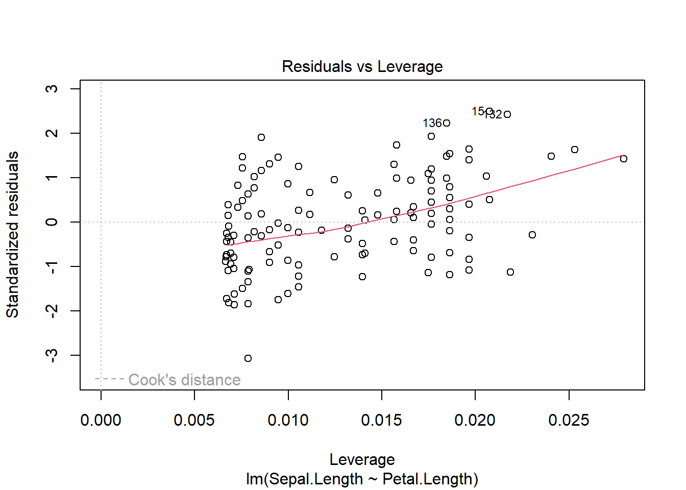
Call:
lm(formula = Sepal.Length ~ Petal.Length, data = iris)

Residuals:
     Min       1Q   Median       3Q      Max
-1.24675 -0.29657 -0.01515  0.27676  1.00269

Coefficients:
             Estimate Std. Error t value Pr(>|t|)
(Intercept)   4.30660    0.07839   54.94   <2e-16 ***
Petal.Length  0.40892    0.01889   21.65   <2e-16 ***
---
Signif. codes:  0 '***' 0.001 '**' 0.01 '*' 0.05 '.' 0.1 ' ' 1

Residual standard error: 0.4071 on 148 degrees of freedom
Multiple R-squared:   0.76, Adjusted R-squared:  0.7583
F-statistic: 468.6 on 1 and 148 DF,  p-value: < 2.2e-16
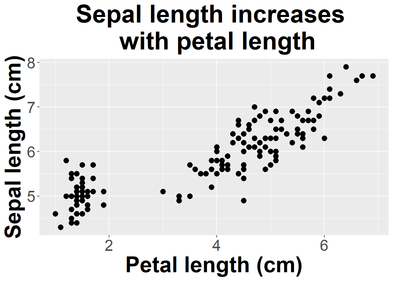
We find that F1,148=468.5, p < 0.01, so we reject the null hypothesis that the slope is equal to 0. The estimate indicates a slope of 0.408, so sepal length increases with petal length. An R2 value of 0.76 indicates petal length explains about 75% of the variation in sepal length.
Alternatively, we could consider if the association between the two variables is equal to 0 (or not).
cor.test(~ Sepal.Length + Petal.Length, data = iris)
    Pearson's product-moment correlation

data:  Sepal.Length and Petal.Length
t = 21.646, df = 148, p-value < 2.2e-16
alternative hypothesis: true correlation is not equal to 0
95 percent confidence interval:
 0.8270363 0.9055080
sample estimates:
      cor
0.8717538
We find the same p-value (using a t-distribution), and see that the estimated linear correlation coefficient, .87, is the square of our R2 value.
If we prefer a rank-based test, we can update the code:
cor.test(~ Sepal.Length + Petal.Length, data = iris,method="spearman")
Warning in cor.test.default(x = mf[[1L]], y = mf[[2L]], ...): Cannot compute
exact p-value with ties
    Spearman's rank correlation rho

data:  Sepal.Length and Petal.Length
S = 66429, p-value < 2.2e-16
alternative hypothesis: true rho is not equal to 0
sample estimates:
      rho
0.8818981
Which again leads us to reject the null hypothesis. Finally, a bootstrap options can be produced
where estimates indicated the slope does not contain 0.
Swirl lesson
Swirl is an R package that provides guided lessons to help you learn and review material. These lessons should serve as a bridge between all the code provided in the slides and background reading and the key functions and concepts from each lesson. A full course lesson (all lessons combined) can also be downloaded using the following instructions.
THIS IS ONE OF THE FEW TIMES I RECOMMEND WORKING DIRECTLY IN THE CONSOLE! THERE IS NO NEED TO DEVELOP A SCRIPT FOR THESE INTERACTIVE SESSIONS, THOUGH YOU CAN!
install the “swirl” package
run the following code once on the computer to install a new course
Is there evidence that age, height, or weight impact change in pulse rate for students who ran (Ran column = 1)? For each of these, how much variation in pulse rate do they explain?
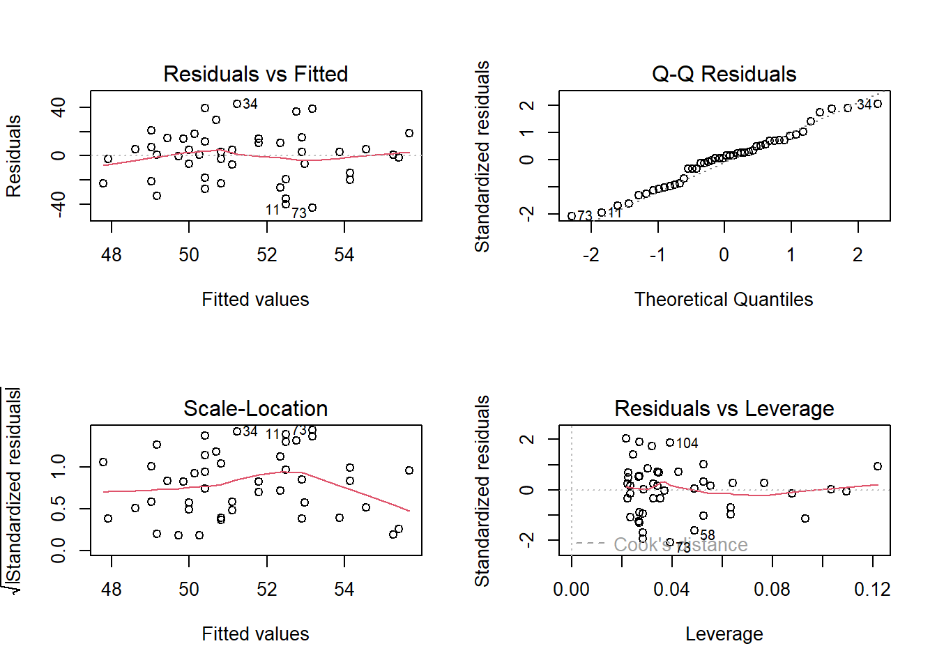
pulse <-read.table("https://raw.githubusercontent.com/jsgosnell/CUNY-BioStats/refs/heads/master/datasets/ms212.txt", header = T, stringsAsFactors = T)pulse$change <- pulse$Pulse2 - pulse$Pulse1#need to make columns entered as numeral change to factor, although it doesn't #really matter when only 2 groups (why?)pulse$Exercise <-as.factor(pulse$Exercise)pulse$Gender <-as.factor(pulse$Gender)#ageexercise <-lm(change ~ Age, pulse[pulse$Ran ==1, ])par(mfrow =c (2,2))plot(exercise)
require(car)Anova(exercise, type ="III")
Anova Table (Type III tests)

Response: change
             Sum Sq Df F value   Pr(>F)
(Intercept)  3882.7  1  8.6317 0.005242 **
Age           222.7  1  0.4950 0.485395
Residuals   19792.3 44
---
Signif. codes:  0 '***' 0.001 '**' 0.01 '*' 0.05 '.' 0.1 ' ' 1
summary(exercise)
Call:
lm(formula = change ~ Age, data = pulse[pulse$Ran == 1, ])

Residuals:
    Min      1Q  Median      3Q     Max
-41.512 -12.183   2.591  12.893  44.868

Coefficients:
            Estimate Std. Error t value Pr(>|t|)
(Intercept)  67.3759    22.9328   2.938  0.00524 **
Age          -0.7932     1.1274  -0.704  0.48539
---
Signif. codes:  0 '***' 0.001 '**' 0.01 '*' 0.05 '.' 0.1 ' ' 1

Residual standard error: 21.21 on 44 degrees of freedom
Multiple R-squared:  0.01113,   Adjusted R-squared:  -0.01135
F-statistic: 0.495 on 1 and 44 DF,  p-value: 0.4854
First we need to make a column that shows change in pulse rate. We also should change Exercise and gender to factors.
For age we note the model meets assumptions (no patterns in residuals and residuals follow a normal distribution). We also find no evidence that age impacts change (F1,44 = .4950, p = 0.49). We fail to reject our null hypothesis that there is no relationship between age and change in pulse rate. We also note that age only explains 1.1% of the variation in change in pulse rate (likely due to chance!).
Call:
lm(formula = change ~ Weight, data = pulse[pulse$Ran == 1, ])

Residuals:
    Min      1Q  Median      3Q     Max
-43.173 -17.343   1.967  13.503  42.760

Coefficients:
            Estimate Std. Error t value Pr(>|t|)
(Intercept)  42.1276    14.9300   2.822  0.00714 **
Weight        0.1381     0.2176   0.635  0.52899
---
Signif. codes:  0 '***' 0.001 '**' 0.01 '*' 0.05 '.' 0.1 ' ' 1

Residual standard error: 21.23 on 44 degrees of freedom
Multiple R-squared:  0.009069,  Adjusted R-squared:  -0.01345
F-statistic: 0.4027 on 1 and 44 DF,  p-value: 0.529
For weight we note the model meets assumptions. We also find no evidence that weight impacts change (F1,44 = .4027, p = 0.53). We fail to reject our null hypothesis that there is no relationship between weight and change in pulse rate. We also note that weight only explains 1% of the variation in change in pulse rate (likely due to chance!).
Anova Table (Type III tests)

Response: change
             Sum Sq Df F value Pr(>F)
(Intercept)   243.9  1  0.5503 0.4621
Height        511.4  1  1.1536 0.2886
Residuals   19503.6 44
summary(exercise)
Call:
lm(formula = change ~ Height, data = pulse[pulse$Ran == 1, ])

Residuals:
    Min      1Q  Median      3Q     Max
-42.798 -17.012   1.848  12.177  43.861

Coefficients:
            Estimate Std. Error t value Pr(>|t|)
(Intercept)  21.0688    28.4017   0.742    0.462
Height        0.1773     0.1650   1.074    0.289

Residual standard error: 21.05 on 44 degrees of freedom
Multiple R-squared:  0.02555,   Adjusted R-squared:  0.003402
F-statistic: 1.154 on 1 and 44 DF,  p-value: 0.2886
For height we note the model meets assumptions. We also find no evidence that weight impacts change (F1,44 = 1.15, p = 0.29). We fail to reject our null hypothesis that there is no relationship between height and change in pulse rate. We also note that age only explains 2.5% of the variation in change in pulse rate (likely due to chance!).
2
(from OZDASL repository,https://gksmyth.github.io/ozdasl/general/stature.html; reference for more information)
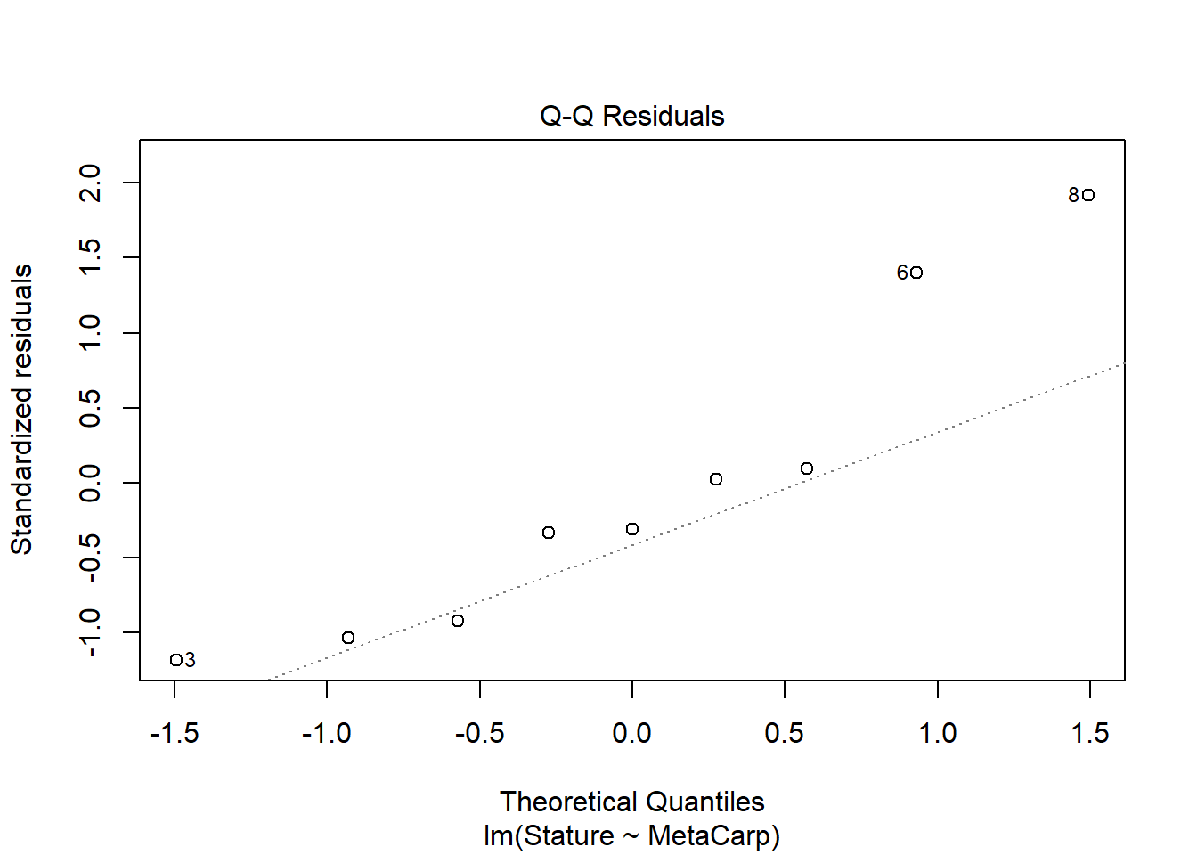
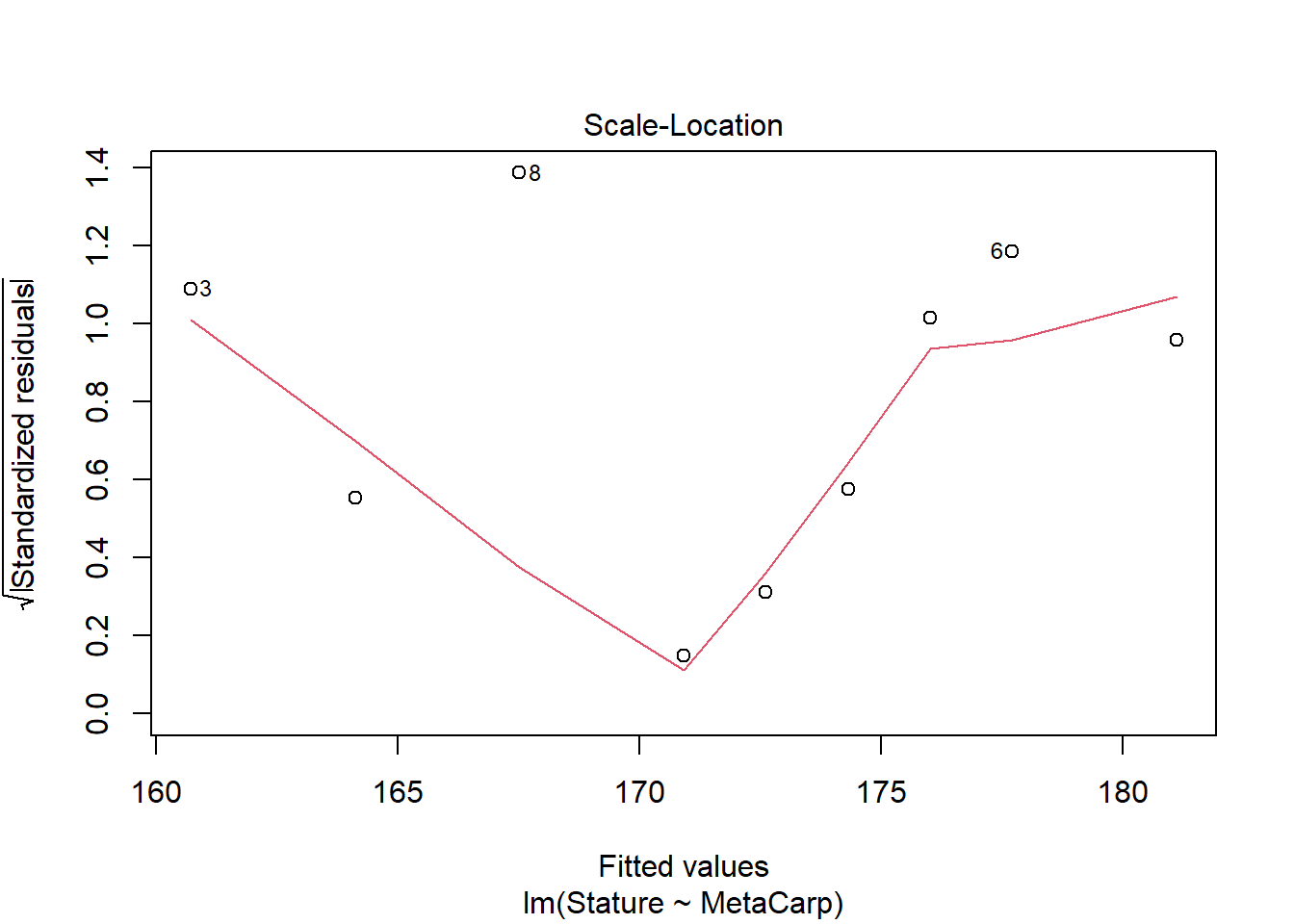
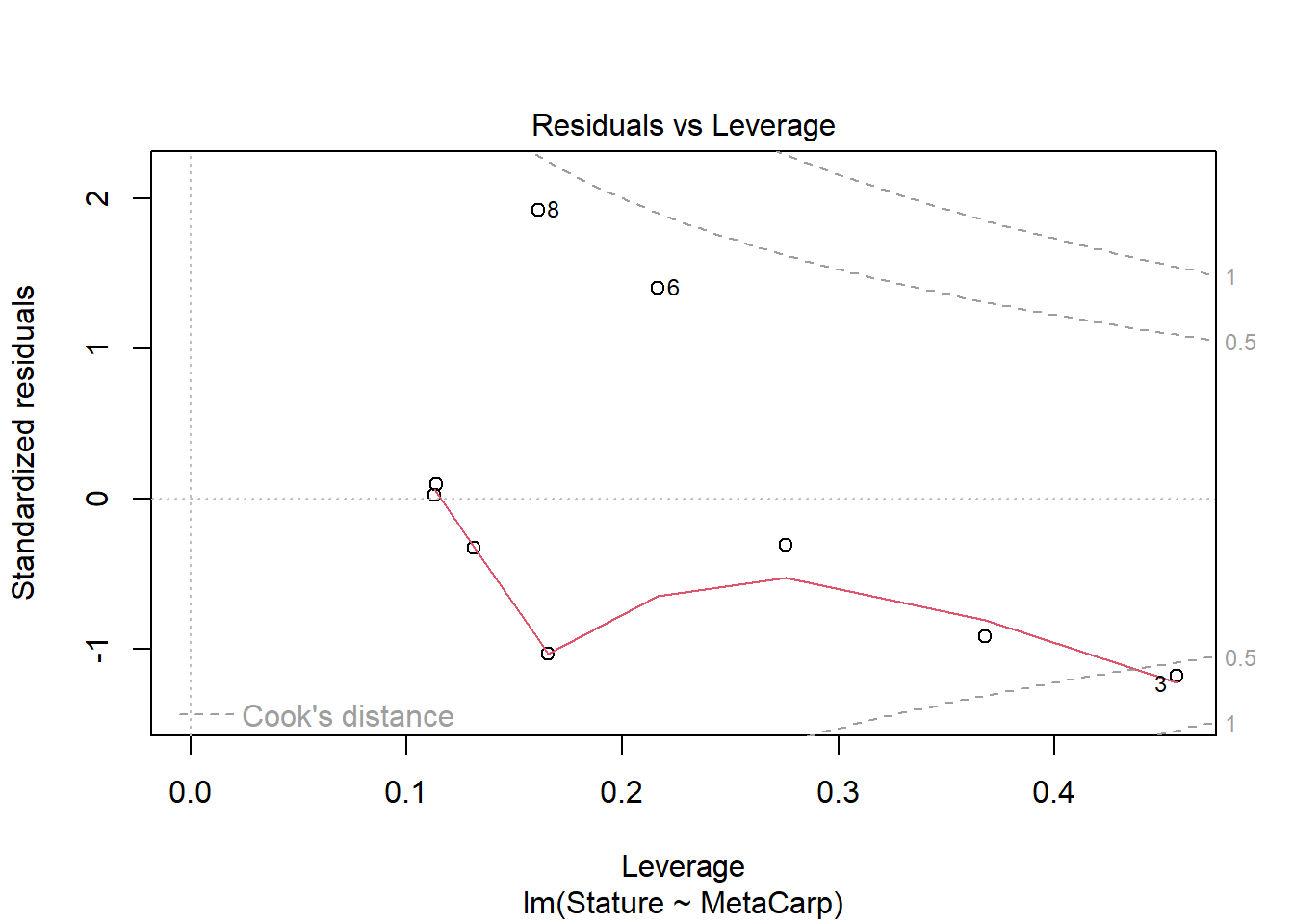
When anthropologists analyze human skeletal remains, an important piece of information is living stature. Since skeletons are commonly based on statistical methods that utilize measurements on small bones. The following data was presented in a paper in the American Journal of Physical Anthropology to validate one such method. Data is available @
as a tab-delimted file (need to use read.table!) Is there evidence that metacarpal bone length is a good predictor of stature? If so, how much variation does it account for in the response variable?
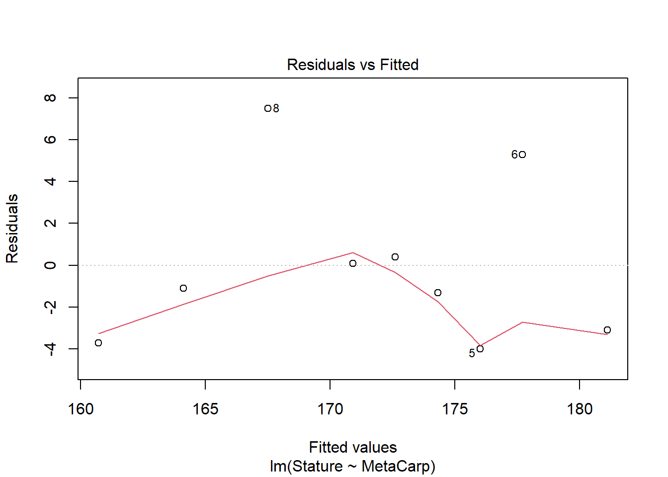
Call:
lm(formula = Stature ~ MetaCarp, data = height)

Residuals:
    Min      1Q  Median      3Q     Max
-4.0102 -3.1091 -1.1128  0.3891  7.4880

Coefficients:
            Estimate Std. Error t value Pr(>|t|)
(Intercept)   94.428     17.691   5.338  0.00108 **
MetaCarp       1.700      0.388   4.380  0.00323 **
---
Signif. codes:  0 '***' 0.001 '**' 0.01 '*' 0.05 '.' 0.1 ' ' 1

Residual standard error: 4.255 on 7 degrees of freedom
Multiple R-squared:  0.7327,    Adjusted R-squared:  0.6945
F-statistic: 19.19 on 1 and 7 DF,  p-value: 0.003234
To consider the relationship among these continuous variables, we used linear regression. Analysis of model assumptions suggest assumptions are met, although the dataset is small. Analysis suggests there is a significant positive relationship between metacarpal length and stature (F1,7 = 19.19, p = 0.003). The R2 value indicates that metacarpal length explains 73% of the variation in stature. Coefficients indicate that stature increases with increasing metacarpal length.
3
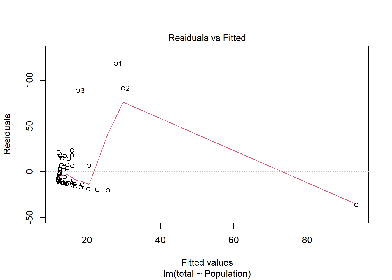
Data on medals won by various countries in the 1992 and 1994 Olympics is available in a tab-delimited file at
Warning in cor.test.default(x = mf[[1L]], y = mf[[2L]], ...): Cannot compute
exact p-value with ties
    Spearman's rank correlation rho

data:  total and Population
S = 29456, p-value = 0.04271
alternative hypothesis: true rho is not equal to 0
sample estimates:
      rho
0.2582412
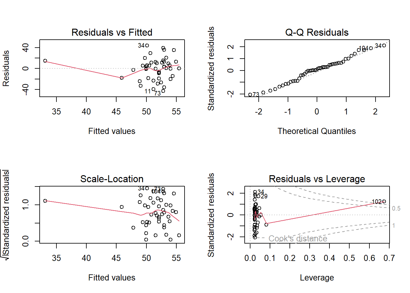
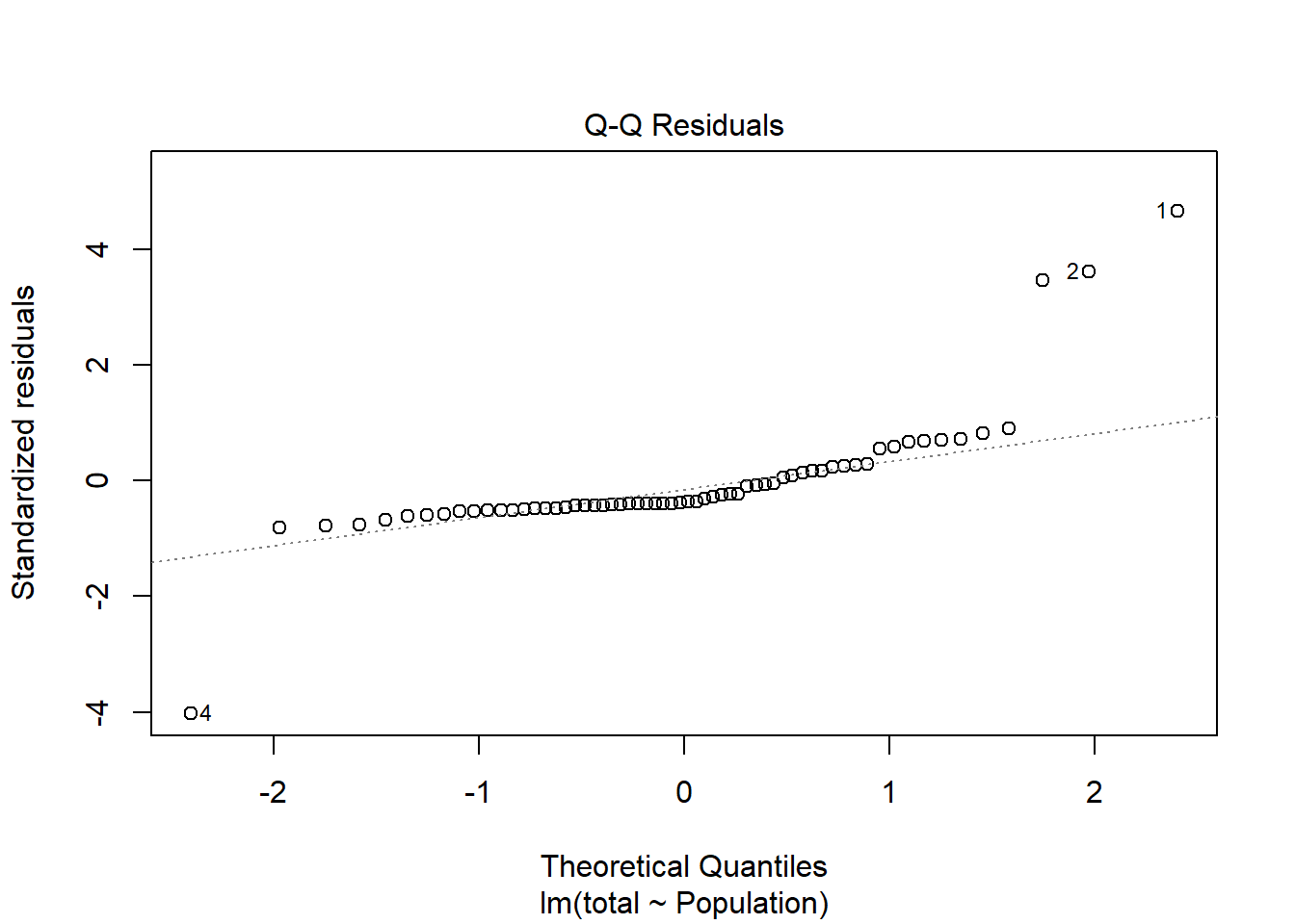
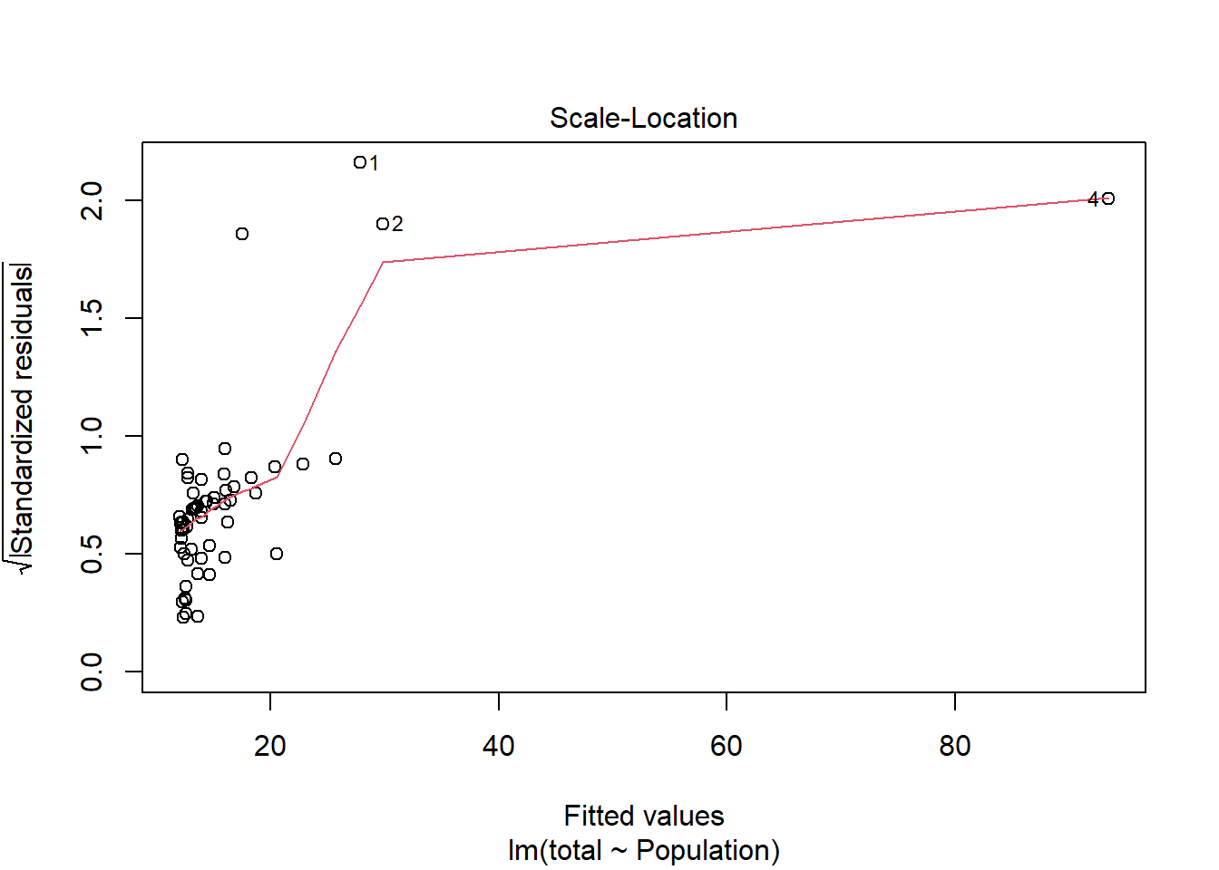
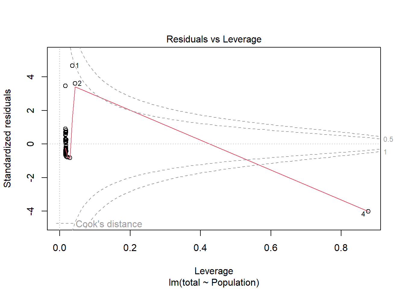
There is a high leverage point in the dataset (row 4), but residuals appear to be fairly normally distributed and little structure exists in the graph of Residuals vs. Fitted Values. Analysis using linear regression suggests a significant ( F1,60 = 10.45, p = 0.002) positive relationship between population size and medal count that explains ~15% of the variation in the response variable. Rank- correlation analysis also indicated this relationship exists.
4
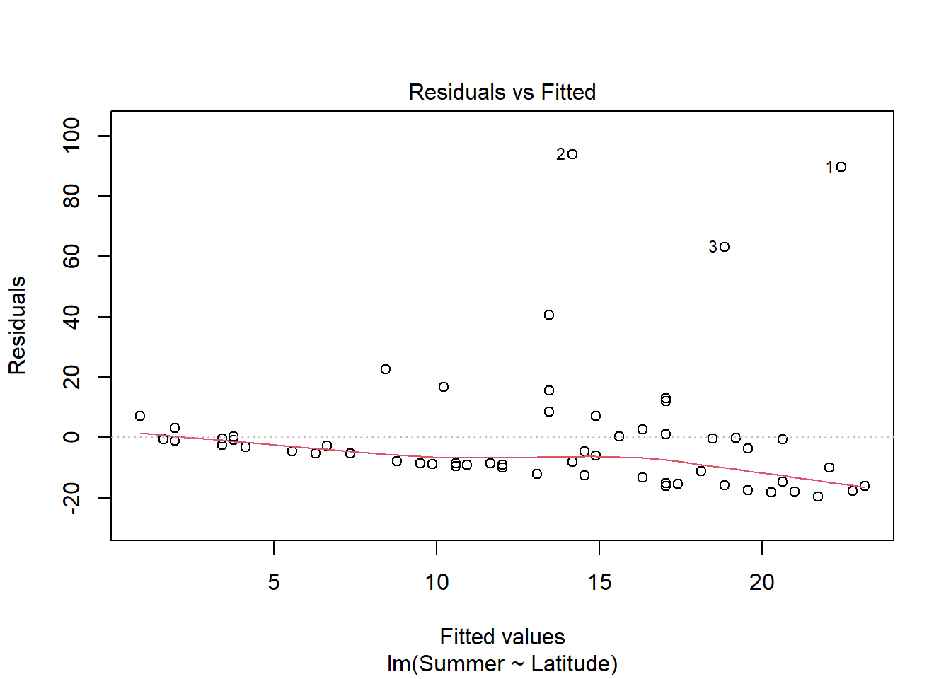
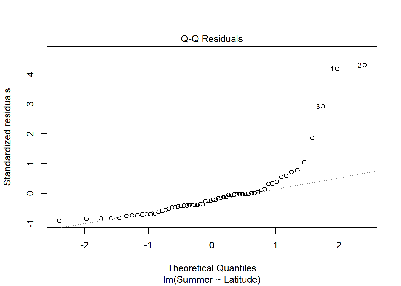
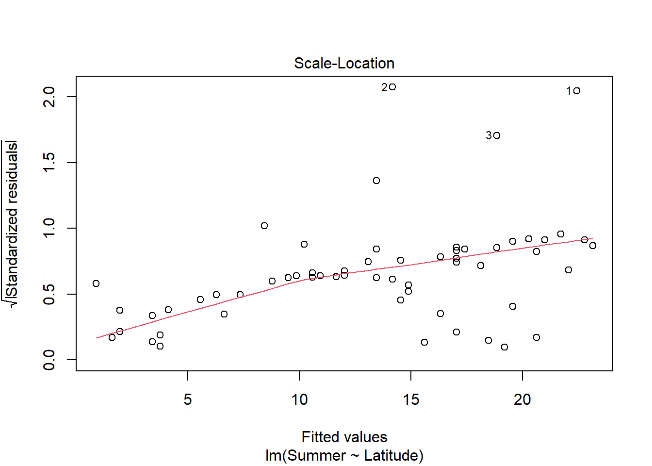
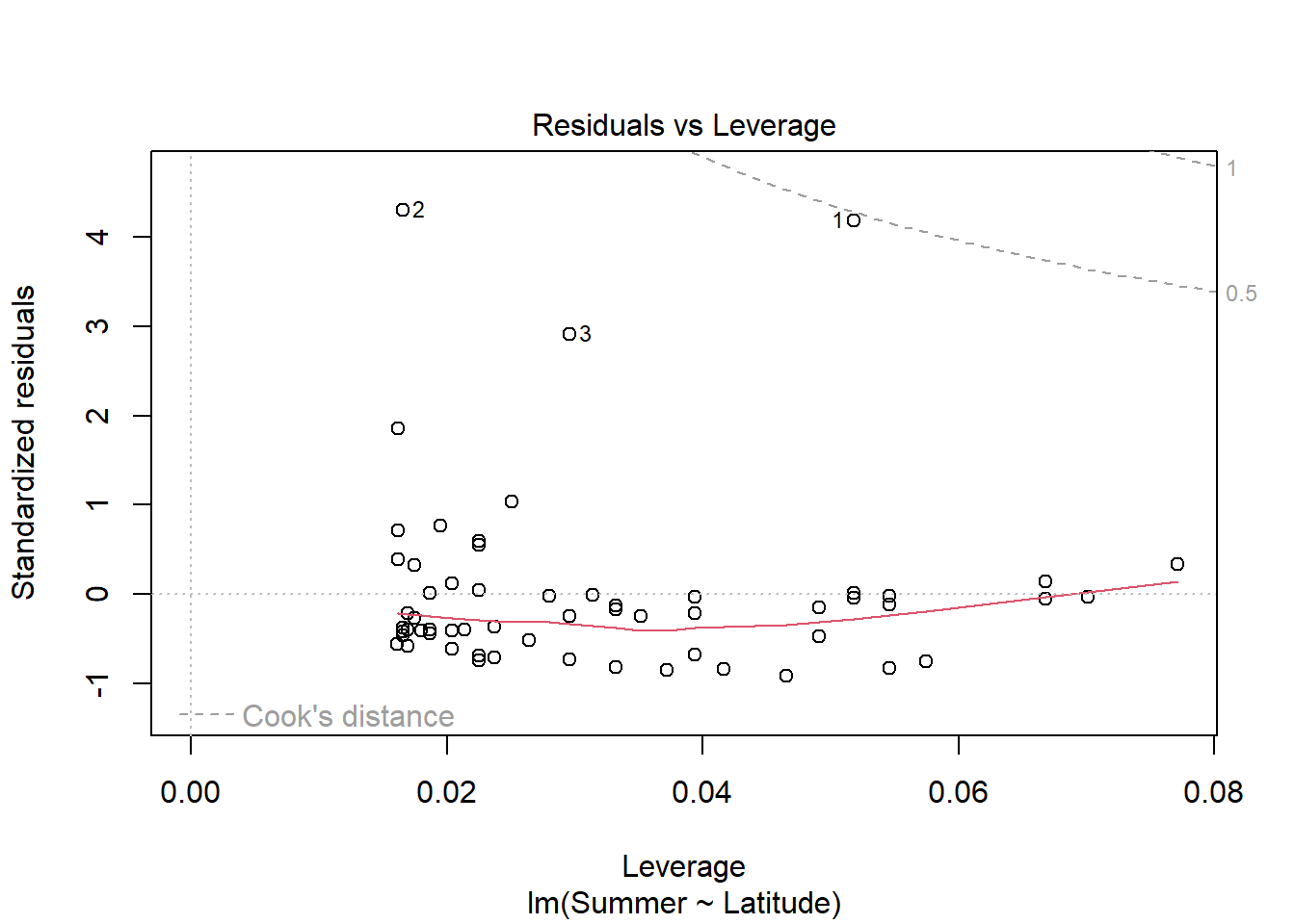
Continuing with the Olympic data, is there a relationship between the latitude of a country and the number of medals won in summer or winter Olympics?
#still using medalssummer_medals <-lm(Summer ~ Latitude, medals)plot(summer_medals)
Anova(summer_medals, type ="III")
Anova Table (Type III tests)

Response: Summer
             Sum Sq Df F value  Pr(>F)
(Intercept)     3.6  1  0.0075 0.93143
Latitude     2440.3  1  5.0389 0.02848 *
Residuals   29057.2 60
---
Signif. codes:  0 '***' 0.001 '**' 0.01 '*' 0.05 '.' 0.1 ' ' 1
summary(summer_medals)
Call:
lm(formula = Summer ~ Latitude, data = medals)

Residuals:
    Min      1Q  Median      3Q     Max
-19.707 -10.856  -4.922   0.352  93.827

Coefficients:
            Estimate Std. Error t value Pr(>|t|)
(Intercept)   0.5403     6.2531   0.086   0.9314
Latitude      0.3588     0.1598   2.245   0.0285 *
---
Signif. codes:  0 '***' 0.001 '**' 0.01 '*' 0.05 '.' 0.1 ' ' 1

Residual standard error: 22.01 on 60 degrees of freedom
Multiple R-squared:  0.07747,   Adjusted R-squared:  0.0621
F-statistic: 5.039 on 1 and 60 DF,  p-value: 0.02848
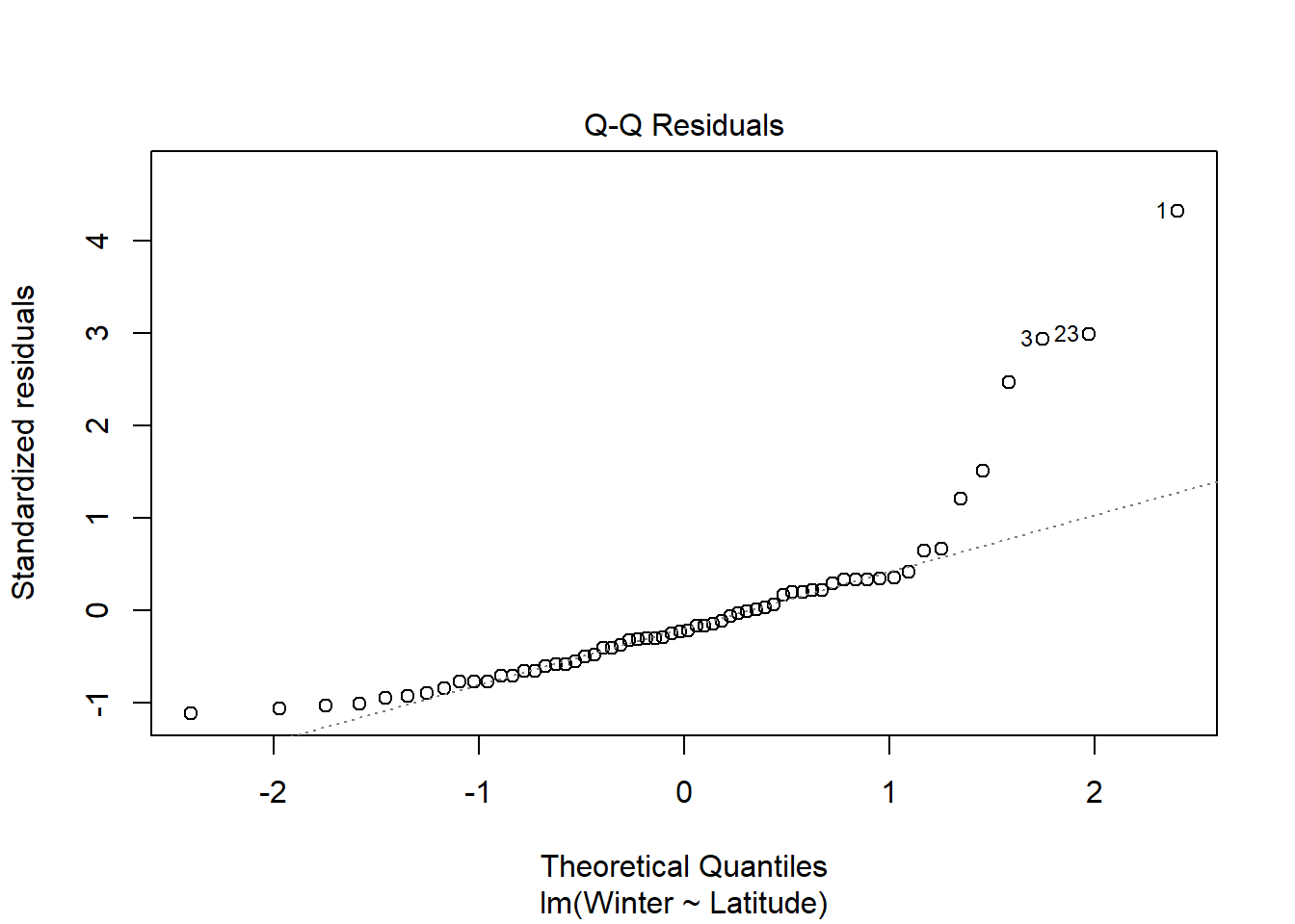
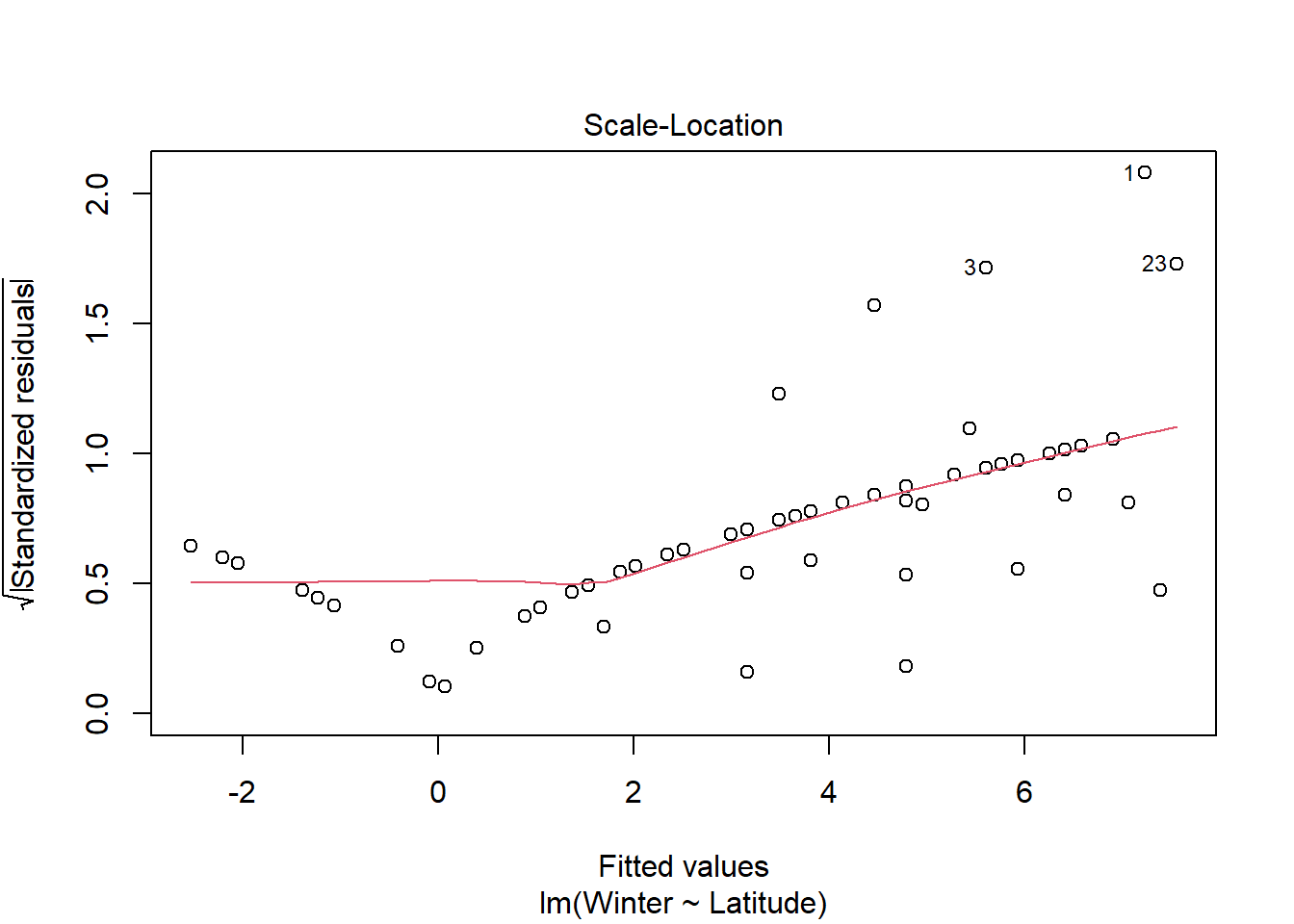
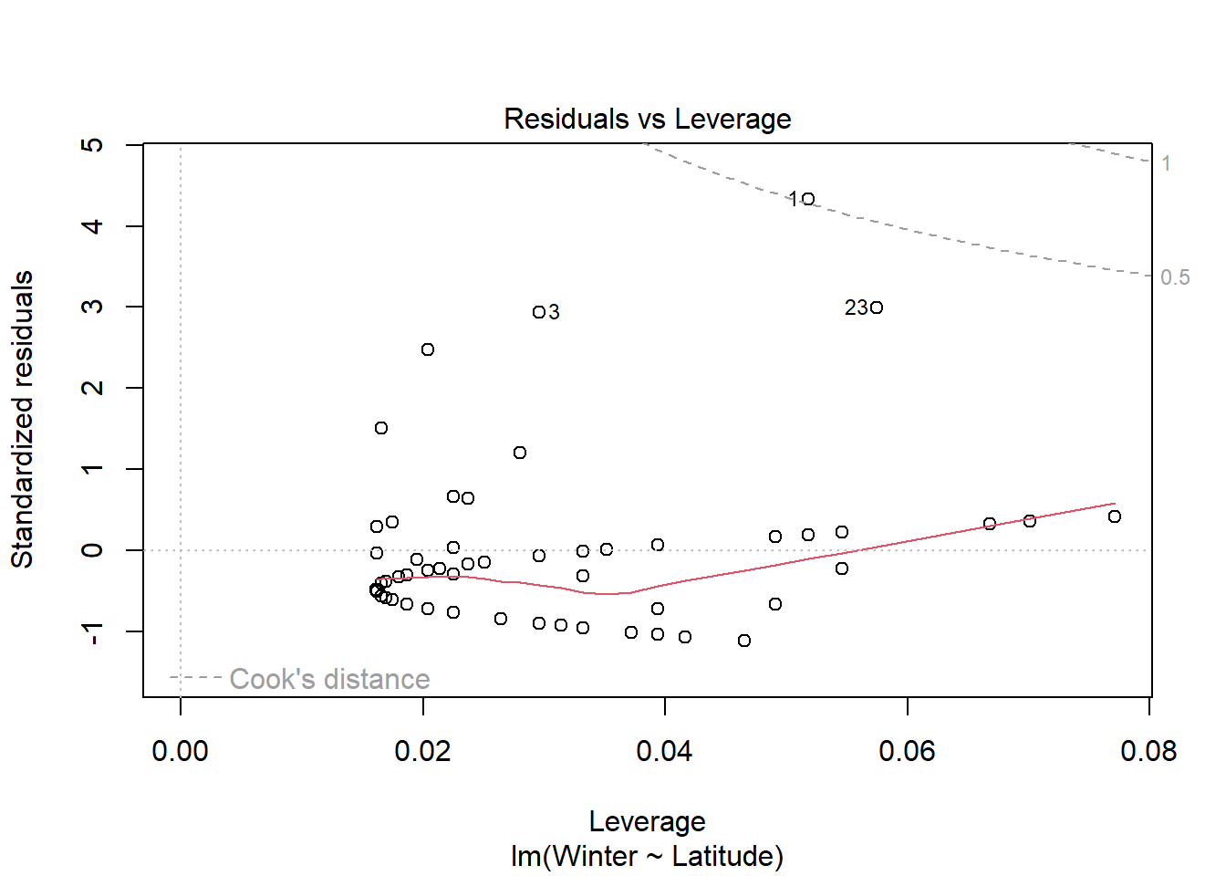
Anova Table (Type III tests)

Response: Winter
             Sum Sq Df F value    Pr(>F)
(Intercept)   90.07  1  2.2353 0.1401300
Latitude     502.29  1 12.4652 0.0008035 ***
Residuals   2417.71 60
---
Signif. codes:  0 '***' 0.001 '**' 0.01 '*' 0.05 '.' 0.1 ' ' 1
summary(winter_medals)
Call:
lm(formula = Winter ~ Latitude, data = medals)

Residuals:
   Min     1Q Median     3Q    Max
-6.906 -3.773 -1.383  1.395 26.768

Coefficients:
            Estimate Std. Error t value Pr(>|t|)
(Intercept)  -2.6967     1.8037  -1.495 0.140130
Latitude      0.1628     0.0461   3.531 0.000803 ***
---
Signif. codes:  0 '***' 0.001 '**' 0.01 '*' 0.05 '.' 0.1 ' ' 1

Residual standard error: 6.348 on 60 degrees of freedom
Multiple R-squared:  0.172, Adjusted R-squared:  0.1582
F-statistic: 12.47 on 1 and 60 DF,  p-value: 0.0008035
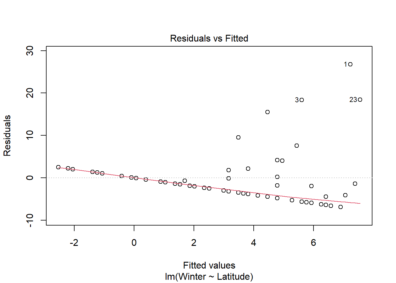
Visual analysis of residuals from both models show some structure in the residual and deviations from normality, but we continue on with linear regression given the small sample size. Both summer and winter medal counts are positively (surpisingly) and significantly (both p <.05) related to latitude, with latitude explaining ~17% of the variation in winter medal count and ~8% of the data in summer medal count.
5
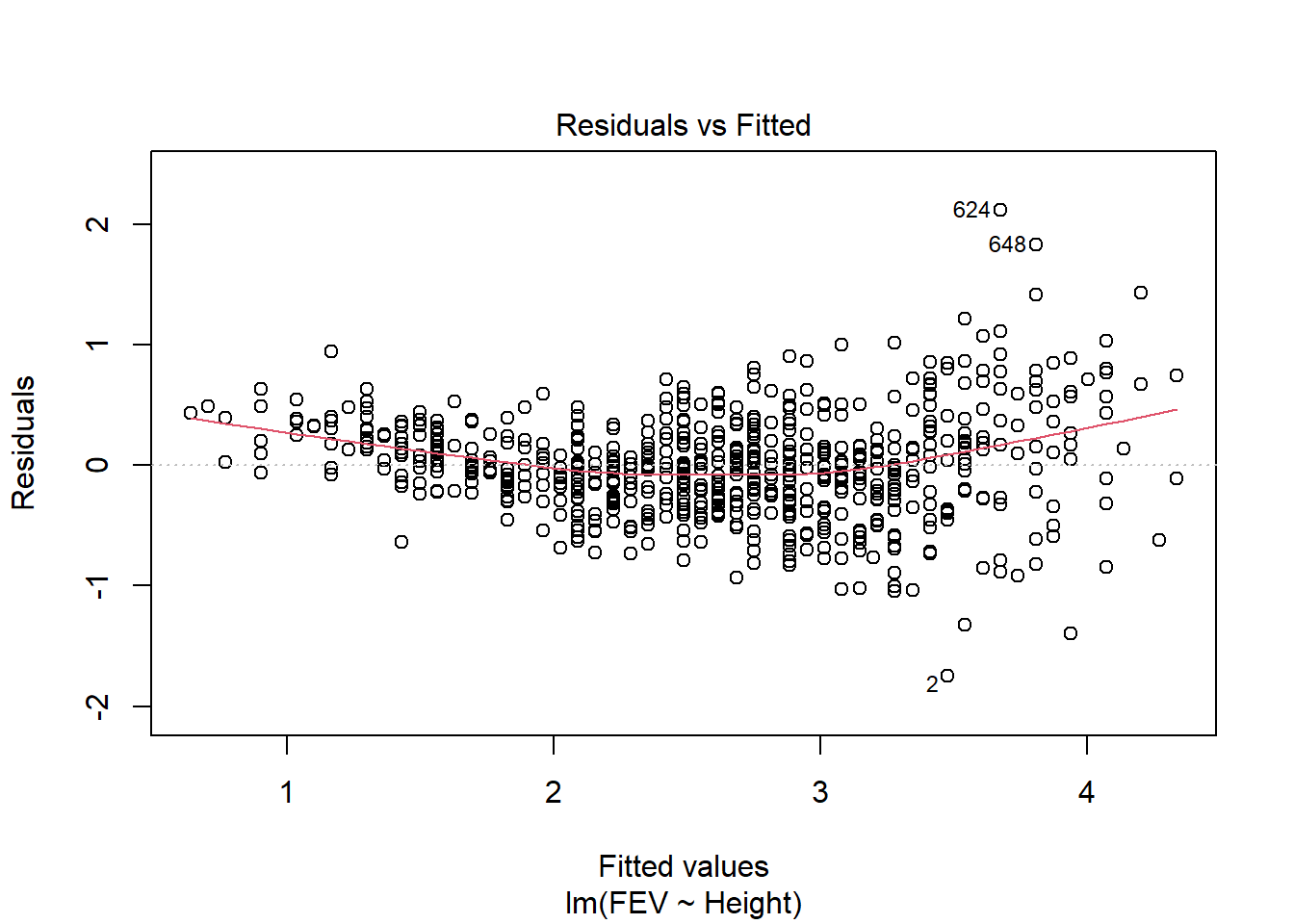
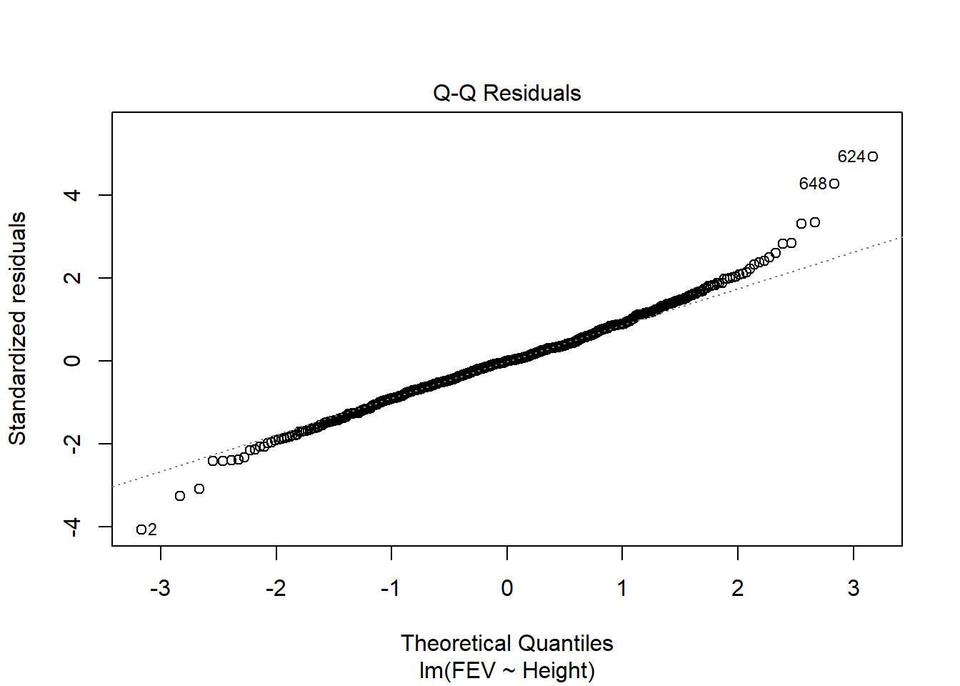
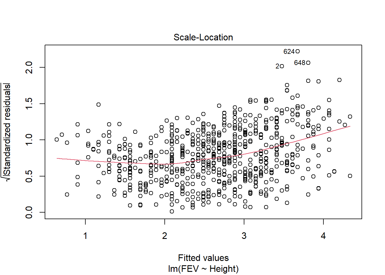
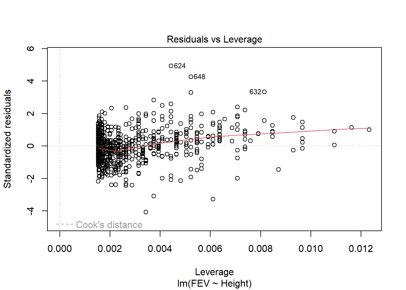
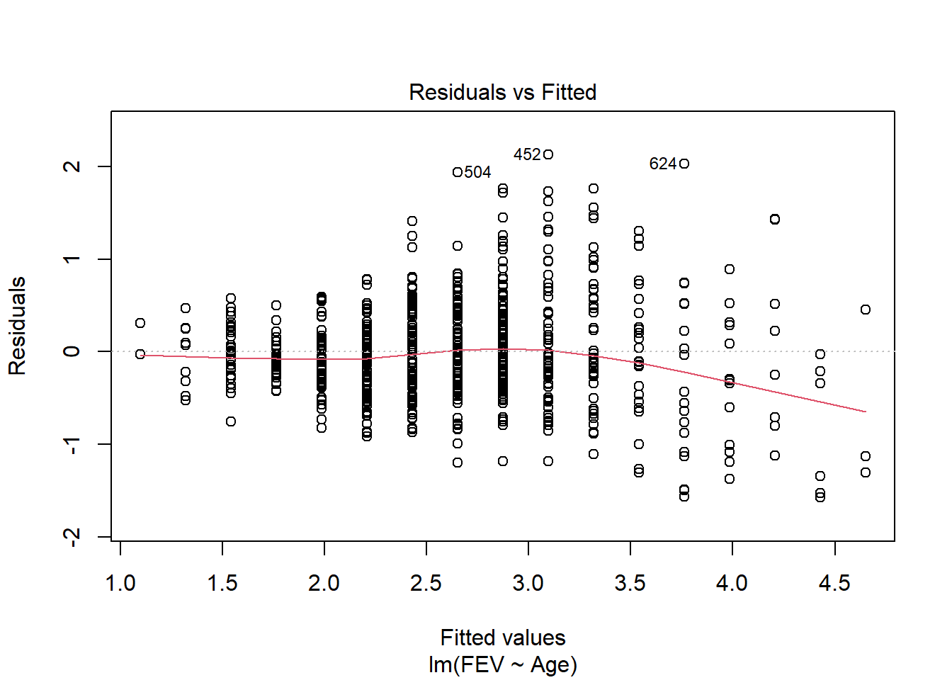
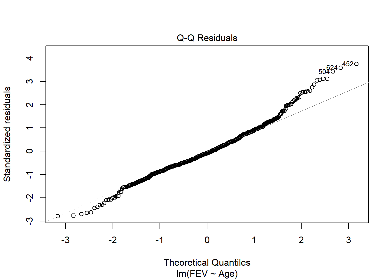
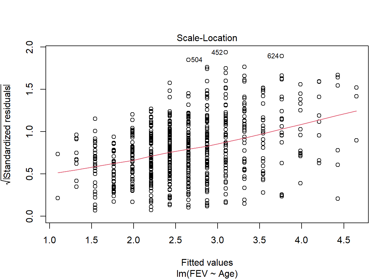
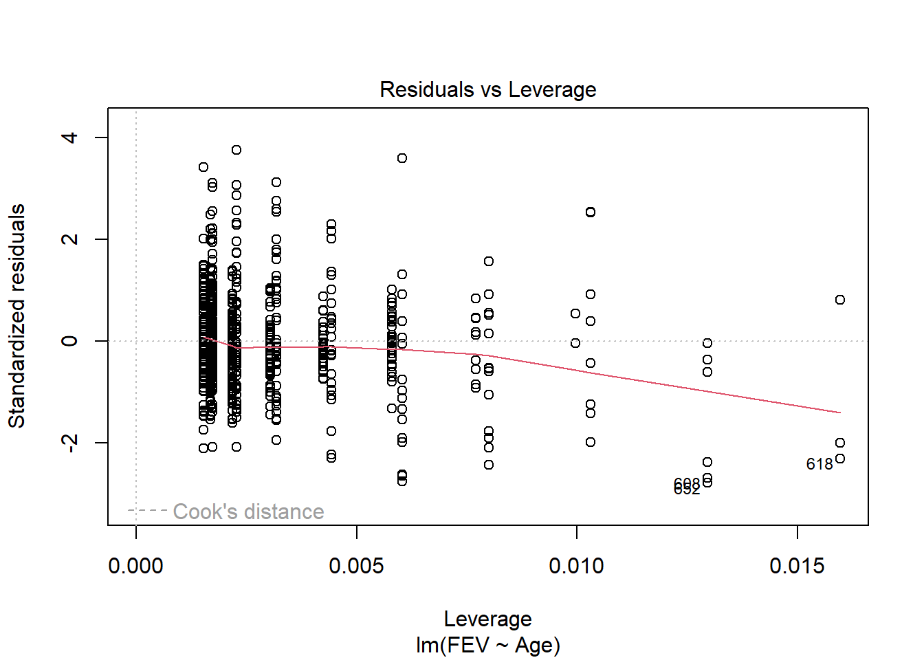
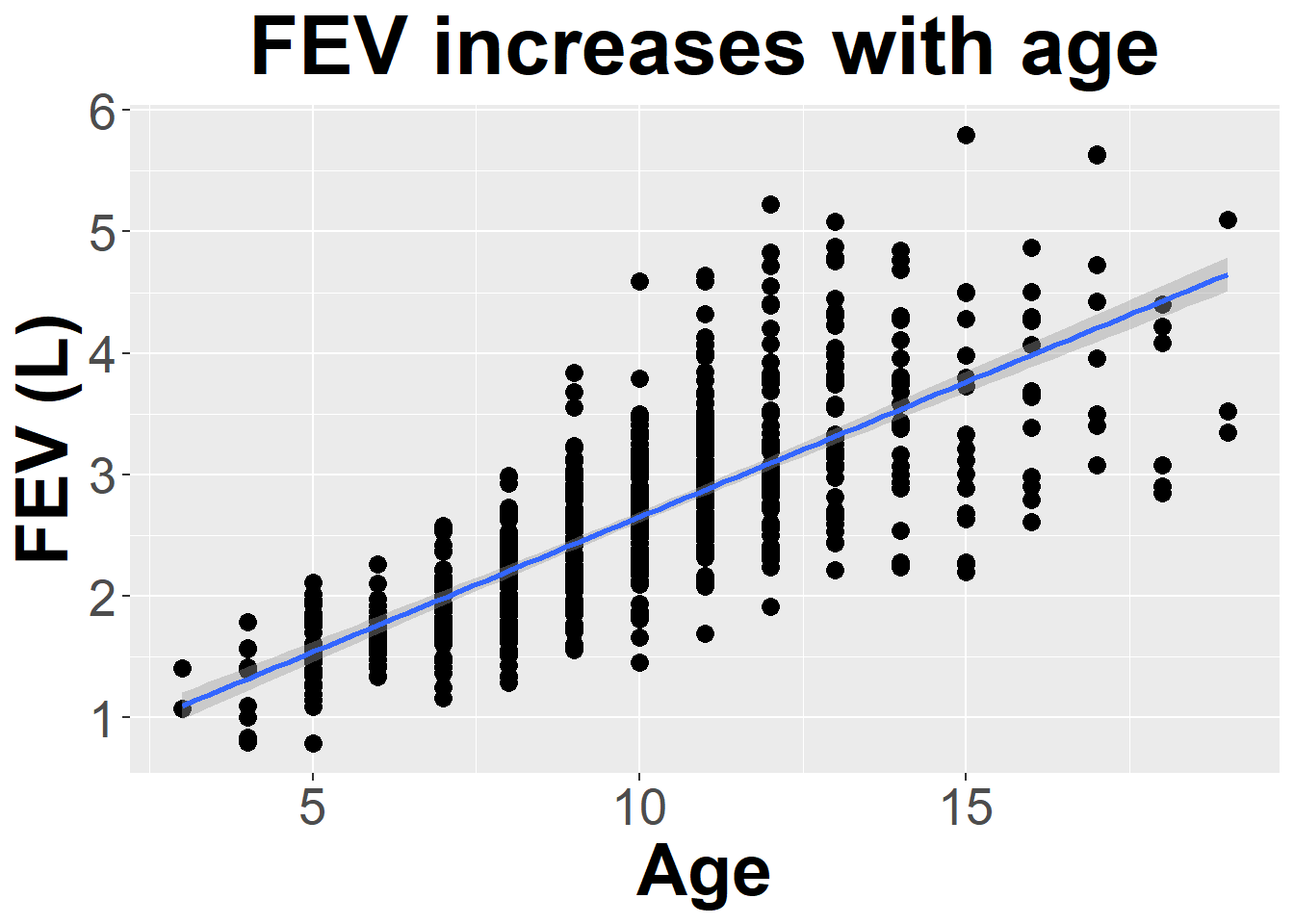
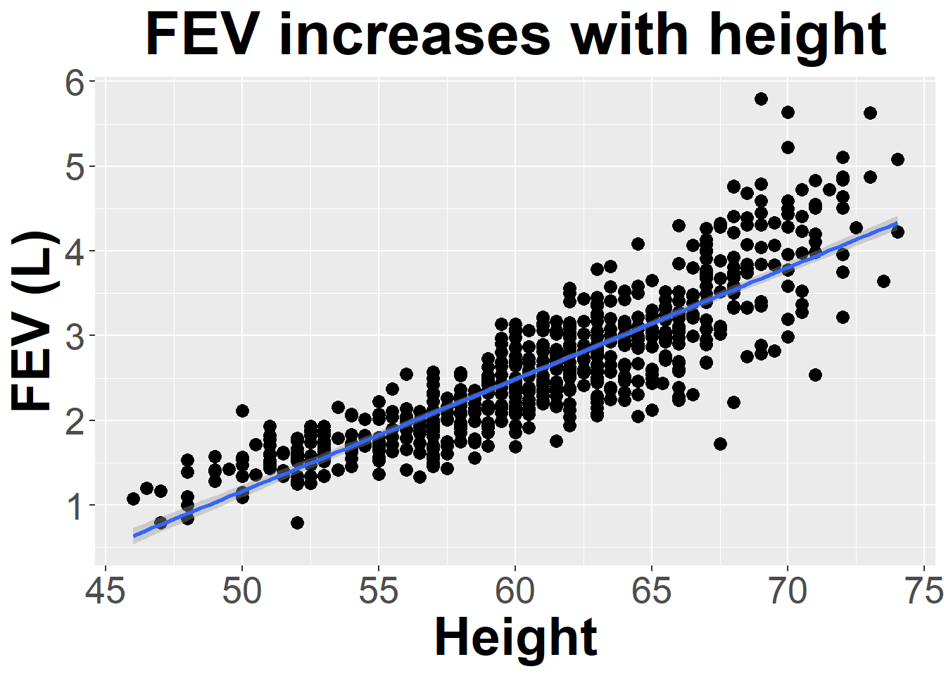
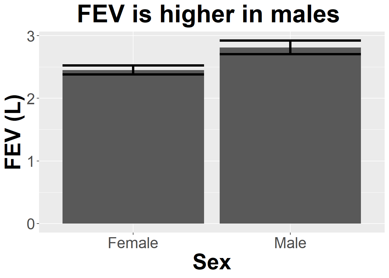
Data on FEV (forced expiratory volume), a measure of lung function, can be found at
    ID Age   FEV Height    Sex Smoker
1  301   9 1.708   57.0 Female    Non
2  451   8 1.724   67.5 Female    Non
3  501   7 1.720   54.5 Female    Non
4  642   9 1.558   53.0   Male    Non
5  901   9 1.895   57.0   Male    Non
6 1701   8 2.336   61.0 Female    Non
Warning: Using `size` aesthetic for lines was deprecated in ggplot2 3.4.0.
ℹ Please use `linewidth` instead.
7
Find an example of a regression or correlation from a paper that is related to your research or a field of interest. Make sure you understand the connections between the methods, results, and graphs. Briefly answer the following questions
What is the name of the paper and who are the authors?
What was the dependent variable?
What were the independent variables?
Was there a relationship between them? If so, describe it (positive, negative).