iris_anova <- lm(Sepal.Length~Species, iris)Compare means among groups
Remember you should
- add code chunks by clicking the Insert Chunk button on the toolbar or by pressing Ctrl+Alt+I to answer the questions!
- use visual mode or render your file to produce a version that you can see!
- render your file to make sure it runs (and that you haven’t been working out of order)
- save your work often
- commit it via git!
- push updates to github
Overview
This practice reviews the Compare means among groups lecture.
Examples
We will run ANOVA’s using the lm function to connect them to other test. First, build the model
Then use the object it created to test assumptions
par(mfrow = c(2,2))
plot(iris_anova)
If assumptions are met, check the p-value using the summary or Anova function.
summary(iris_anova)
Call:
lm(formula = Sepal.Length ~ Species, data = iris)

Residuals:
    Min      1Q  Median      3Q     Max
-1.6880 -0.3285 -0.0060  0.3120  1.3120

Coefficients:
                  Estimate Std. Error t value Pr(>|t|)
(Intercept)         5.0060     0.0728  68.762  < 2e-16 ***
Speciesversicolor   0.9300     0.1030   9.033 8.77e-16 ***
Speciesvirginica    1.5820     0.1030  15.366  < 2e-16 ***
---
Signif. codes:  0 '***' 0.001 '**' 0.01 '*' 0.05 '.' 0.1 ' ' 1

Residual standard error: 0.5148 on 147 degrees of freedom
Multiple R-squared:  0.6187,    Adjusted R-squared:  0.6135
F-statistic: 119.3 on 2 and 147 DF, p-value: < 2.2e-16library(car)Warning: package 'car' was built under R version 4.4.1Loading required package: carDataAnova(iris_anova, type = "III")Anova Table (Type III tests)
Response: Sepal.Length
Sum Sq Df F value Pr(>F)
(Intercept) 1253.00 1 4728.16 < 2.2e-16 ***
Species 63.21 2 119.26 < 2.2e-16 ***
Residuals 38.96 147
---
Signif. codes: 0 '***' 0.001 '**' 0.01 '*' 0.05 '.' 0.1 ' ' 1If the overall test is significant, carry out post hoc tests (Tukey shown here for all pairs, as most common)
library(multcomp)Loading required package: mvtnormLoading required package: survivalLoading required package: TH.dataLoading required package: MASS
Attaching package: 'TH.data'The following object is masked from 'package:MASS':
geysercompare_cont_tukey <- glht(iris_anova, linfct = mcp(Species = "Tukey"))
summary(compare_cont_tukey)
     Simultaneous Tests for General Linear Hypotheses

Multiple Comparisons of Means: Tukey Contrasts


Fit: lm(formula = Sepal.Length ~ Species, data = iris)

Linear Hypotheses:
                            Estimate Std. Error t value Pr(>|t|)
versicolor - setosa == 0       0.930      0.103   9.033   <1e-06 ***
virginica - setosa == 0        1.582      0.103  15.366   <1e-06 ***
virginica - versicolor == 0    0.652      0.103   6.333   <1e-06 ***
---
Signif. codes:  0 '***' 0.001 '**' 0.01 '*' 0.05 '.' 0.1 ' ' 1
(Adjusted p values reported -- single-step method)
Note a special case of an ANOVA (which is a special case of a linear model) is when we only are comparing 2 populations. When this happens, we have a t-test. For example, we can compare only I. virginica and I. setosa.
not_versicolor <- iris[iris$Species != "versicolor",]
t.test(Sepal.Length ~ Species, not_versicolor)
    Welch Two Sample t-test

data:  Sepal.Length by Species
t = -15.386, df = 76.516, p-value < 2.2e-16
alternative hypothesis: true difference in means between group setosa and group virginica is not equal to 0
95 percent confidence interval:
 -1.78676 -1.37724
sample estimates:
   mean in group setosa mean in group virginica
                  5.006                   6.588
If you compare lm and ANOVA output, it may look slightly different.
summary(lm(Sepal.Length ~ Species, not_versicolor))
Call:
lm(formula = Sepal.Length ~ Species, data = not_versicolor)

Residuals:
    Min      1Q  Median      3Q     Max
-1.6880 -0.2880 -0.0060  0.2985  1.3120

Coefficients:
                 Estimate Std. Error t value Pr(>|t|)
(Intercept)        5.0060     0.0727   68.85   <2e-16 ***
Speciesvirginica   1.5820     0.1028   15.39   <2e-16 ***
---
Signif. codes:  0 '***' 0.001 '**' 0.01 '*' 0.05 '.' 0.1 ' ' 1

Residual standard error: 0.5141 on 98 degrees of freedom
Multiple R-squared:  0.7072,    Adjusted R-squared:  0.7042
F-statistic: 236.7 on 1 and 98 DF,  p-value: < 2.2e-16
That’s because by default the t-test does not assume equal variances. We can fix that.
t.test(Sepal.Length ~ Species, not_versicolor, var.equal=T)
    Two Sample t-test

data:  Sepal.Length by Species
t = -15.386, df = 98, p-value < 2.2e-16
alternative hypothesis: true difference in means between group setosa and group virginica is not equal to 0
95 percent confidence interval:
 -1.786042 -1.377958
sample estimates:
   mean in group setosa mean in group virginica
                  5.006                   6.588
but in this case it has minimal impact.
If assumptions are not met, we can use the Kruskal Wallis non-parametric test and associated post hoc tests.
kruskal.test(Sepal.Length ~ Species, data = iris)
    Kruskal-Wallis rank sum test

data:  Sepal.Length by Species
Kruskal-Wallis chi-squared = 96.937, df = 2, p-value < 2.2e-16pairwise.wilcox.test(iris$Sepal.Length,
iris$Species,
p.adjust.method="holm")
Pairwise comparisons using Wilcoxon rank sum test with continuity correction
data: iris$Sepal.Length and iris$Species
setosa versicolor
versicolor 1.7e-13 -
virginica < 2e-16 5.9e-07
P value adjustment method: holm or a bootstrap alternative
library(WRS2)
t1waybt(Sepal.Length~Species, iris)Call:
t1waybt(formula = Sepal.Length ~ Species, data = iris)
Effective number of bootstrap samples was 599.
Test statistic: 111.9502
p-value: 0
Variance explained: 0.716
Effect size: 0.846 bootstrap_post_hoc <- mcppb20(Sepal.Length~Species, iris)
p.adjust(as.numeric(bootstrap_post_hoc$comp[,6]), "holm")[1] 0 0 0For 2 groups, the boot.t.test function in the MKinfer package is also an option.
library(MKinfer)
boot.t.test(Sepal.Length ~ Species, not_versicolor)
Bootstrap Welch Two Sample t-test
data: Sepal.Length by Species
number of bootstrap samples: 9999
bootstrap p-value < 1e-04
bootstrap difference of means (SE) = -1.580476 (0.1015809)
95 percent bootstrap percentile confidence interval:
-1.780 -1.378
Results without bootstrap:
t = -15.386, df = 76.516, p-value < 2.2e-16
alternative hypothesis: true difference in means is not equal to 0
95 percent confidence interval:
-1.78676 -1.37724
sample estimates:
mean in group setosa mean in group virginica
5.006 6.588 A final option (shown here for 2 groups) is to use permutation tests. These tests work by rearranging the data in all (theoretically) possible ways and calculating signals for each permutation. You can then compare what we actually found to that to obtain p-values. Often times we can’t find all the combinations there are too many!), but a good sample (10,000+) should work. The function that we’ll use for this is independence_test from the coin package. It uses the same arguments as the t-test (including the formula interface).
library(coin)
independence_test(Sepal.Length ~ Species, not_versicolor)
Asymptotic General Independence Test
data: Sepal.Length by Species (setosa, virginica)
Z = -8.3675, p-value < 2.2e-16
alternative hypothesis: two.sidedSwirl lesson
Swirl is an R package that provides guided lessons to help you learn and review material. These lessons should serve as a bridge between all the code provided in the slides and background reading and the key functions and concepts from each lesson. A full course lesson (all lessons combined) can also be downloaded using the following instructions.
THIS IS ONE OF THE FEW TIMES I RECOMMEND WORKING DIRECTLY IN THE CONSOLE! THERE IS NO NEED TO DEVELOP A SCRIPT FOR THESE INTERACTIVE SESSIONS, THOUGH YOU CAN!
install the “swirl” package
run the following code once on the computer to install a new course
library(swirl) install_course_github("jsgosnell", "JSG_swirl_lessons")start swirl!
swirl()- swirl()
then follow the on-screen prompts to select the JSG_swirl_lessons course and the lessons you want
- Here we will focus on the Compare means among groups lesson
TIP: If you are seeing duplicate courses (or odd versions of each), you can clear all courses and then re-download the courses by
exiting swirl using escape key or bye() function
bye()uninstalling and reinstalling courses
uninstall_all_courses() install_course_github("jsgosnell", "JSG_swirl_lessons")when you restart swirl with swirl(), you may need to select
- No. Let me start something new
Just for practice
For the following questions, you will use multiple methods to analyze a single dataset. This is for practice and so you can compare! For actual analysis you should only use the best method!
1
Use the iris dataset in R to determine if petal length differs among species. Do this problem using the following methods
ANOVA
Kruskal-Wallis
bootstrapping
Make sure you can plot the data and carry out multiple comparison methods as needed. Also be sure to understand the use of coefficients and adjusted R2 values and where to find them.
#plot
library(Rmisc)Loading required package: latticeLoading required package: plyrfunction_output <- summarySE(iris, measurevar="Petal.Length", groupvars =
c("Species"))
library(ggplot2)
ggplot(function_output, aes(x=Species, y=Petal.Length)) +
geom_col(aes(fill=Species), size = 3) +
geom_errorbar(aes(ymin=Petal.Length-ci, ymax=Petal.Length+ci), size=1.5) +
ylab("Petal Length (cm)")+ggtitle("Petal Length of \n various iris species")+
theme(axis.title.x = element_text(face="bold", size=28),
axis.title.y = element_text(face="bold", size=28),
axis.text.y = element_text(size=20),
axis.text.x = element_text(size=20),
legend.text =element_text(size=20),
legend.title = element_text(size=20, face="bold"),
plot.title = element_text(hjust = 0.5, face="bold", size=32))Warning: Using `size` aesthetic for lines was deprecated in ggplot2 3.4.0.
ℹ Please use `linewidth` instead.
petal <- lm(Petal.Length ~ Species, iris)
plot(petal)


library(car)
Anova(petal, type = "III")Anova Table (Type III tests)
Response: Petal.Length
Sum Sq Df F value Pr(>F)
(Intercept) 106.87 1 577.1 < 2.2e-16 ***
Species 437.10 2 1180.2 < 2.2e-16 ***
Residuals 27.22 147
---
Signif. codes: 0 '***' 0.001 '**' 0.01 '*' 0.05 '.' 0.1 ' ' 1#compare to
summary(petal)
Call:
lm(formula = Petal.Length ~ Species, data = iris)
Residuals:
Min 1Q Median 3Q Max
-1.260 -0.258 0.038 0.240 1.348
Coefficients:
Estimate Std. Error t value Pr(>|t|)
(Intercept) 1.46200 0.06086 24.02 <2e-16 ***
Speciesversicolor 2.79800 0.08607 32.51 <2e-16 ***
Speciesvirginica 4.09000 0.08607 47.52 <2e-16 ***
---
Signif. codes: 0 '***' 0.001 '**' 0.01 '*' 0.05 '.' 0.1 ' ' 1
Residual standard error: 0.4303 on 147 degrees of freedom
Multiple R-squared: 0.9414, Adjusted R-squared: 0.9406
F-statistic: 1180 on 2 and 147 DF, p-value: < 2.2e-16library(multcomp)
comp_cholest <- glht(petal, linfct = mcp(Species = "Tukey"))
summary(comp_cholest)
Simultaneous Tests for General Linear Hypotheses
Multiple Comparisons of Means: Tukey Contrasts
Fit: lm(formula = Petal.Length ~ Species, data = iris)
Linear Hypotheses:
Estimate Std. Error t value Pr(>|t|)
versicolor - setosa == 0 2.79800 0.08607 32.51 <2e-16 ***
virginica - setosa == 0 4.09000 0.08607 47.52 <2e-16 ***
virginica - versicolor == 0 1.29200 0.08607 15.01 <2e-16 ***
---
Signif. codes: 0 '***' 0.001 '**' 0.01 '*' 0.05 '.' 0.1 ' ' 1
(Adjusted p values reported -- single-step method)#kw approach
petal <- kruskal.test(Petal.Length ~ Species, iris)
pairwise.wilcox.test(iris$Sepal.Length,
                          iris$Species,
                          p.adjust.method="holm")
    Pairwise comparisons using Wilcoxon rank sum test with continuity correction

data:  iris$Sepal.Length and iris$Species

           setosa  versicolor
versicolor 1.7e-13 -
virginica  < 2e-16 5.9e-07

P value adjustment method: holm #bootstrap
library(WRS2)
t1waybt(Petal.Length~Species, iris)Call:
t1waybt(formula = Petal.Length ~ Species, data = iris)
Effective number of bootstrap samples was 599.
Test statistic: 1510.684
p-value: 0
Variance explained: 0.71
Effect size: 0.843 bootstrap_post_hoc <- mcppb20(Petal.Length~Species, iris)
#use p.adjust to correct for FWER
p.adjust(as.numeric(bootstrap_post_hoc$comp[,6]), "holm")[1] 0 0 0Answer: We used an ANOVA (a special case of linear models) to investigate how a numerical response variable differed among 3 groups. This was appropriate as evidenced by the residual plots (there is no pattern in the residuals and they are normally distributed), but other methods are demonstrated as well.
Using an ANOVA, we found F2,147= 1180.2, which led to a p-value of <.001. Given this, I reject the null hypothesis there is no difference among mean measurements for each species.
Post-hoc testing indicated all species significantly differed from all others (all p <.05) using a Tukey approach to control for family-wise error rate. Kruskal-Wallis and bootstrapping approaches led to similar conclusions.
2
Data on plant heights (in cm) for plants grown with a new and old formulation of fertilizer can be found at
Analyze this data using the t.test function and the lm function to convince yourself that t-tests are special cases of ANOVAs, which are special cases of linear models!
fertilizer <- read.csv("https://docs.google.com/spreadsheets/d/e/2PACX-1vSUVowOKlmTic4ekL7LSbwDcqrsDSXv5K_c4Qyfcvz1lLE1_iINmGzy0zMGxY7z5DImlUErK4S2wY7Y/pub?gid=0&single=true&output=csv",
                       stringsAsFactors = T)
#note use of var.equal!  assumption of ANOVAs
t.test(height ~ fertilizer, fertilizer, var.equal = T)
    Two Sample t-test

data:  height by fertilizer
t = 2.9884, df = 16, p-value = 0.008686
alternative hypothesis: true difference in means between group new and group old is not equal to 0
95 percent confidence interval:
 1.34853 7.93147
sample estimates:
mean in group new mean in group old
            56.55             51.91
fert_lm <- lm(height ~ fertilizer, fertilizer)
plot(fert_lm)


summary(fert_lm)
Call:
lm(formula = height ~ fertilizer, data = fertilizer)

Residuals:
   Min     1Q Median     3Q    Max
 -4.25  -2.61  -0.21   2.38   6.39

Coefficients:
              Estimate Std. Error t value Pr(>|t|)
(Intercept)     56.550      1.157  48.865  < 2e-16 ***
fertilizerold   -4.640      1.553  -2.988  0.00869 **
---
Signif. codes:  0 '***' 0.001 '**' 0.01 '*' 0.05 '.' 0.1 ' ' 1

Residual standard error: 3.273 on 16 degrees of freedom
Multiple R-squared:  0.3582,    Adjusted R-squared:  0.3181
F-statistic: 8.931 on 1 and 16 DF, p-value: 0.008686require(car)
Anova(fert_lm, type = "III")Anova Table (Type III tests)
Response: height
Sum Sq Df F value Pr(>F)
(Intercept) 25583.2 1 2387.7612 < 2.2e-16 ***
fertilizer 95.7 1 8.9308 0.008686 **
Residuals 171.4 16
---
Signif. codes: 0 '***' 0.001 '**' 0.01 '*' 0.05 '.' 0.1 ' ' 1Answer: t-tests and ANOVA (lm) approaches yield the same results. Note for the tests to match exactly we have to assume equal variances among groups for the t-tests. In both we reject the null hypothesis of no difference among mean height of plants based on fertilizer. Notice the t statistic (2.9884) is the square root of the F statistic (8.931). The t distribution corresponds to the F with only 1 df in the numerator (so its not listed!).
For the following questions, pick the appropriate method for analyzing the question. Use a plot of the data and/or model analysis to justify your decision. Make sure you can carry out multiple comparison methods as needed. Also be sure to understand the use of coefficients and adjusted R2 values and where to find them.
3
Data on sugar cane yield for multiple fields is available using
read.table("https://raw.githubusercontent.com/jsgosnell/CUNY-BioStats/refs/heads/master/datasets/cane.txt", header = T, stringsAsFactors = T) District DistrictGroup DistrictPosition SoilID
1 PineCreek Cairns/Mulgrave(dry) S 838
2 NorthBarron NorthCairns N 802
3 NorthBarron NorthCairns N 802
4 NorthBarron NorthCairns N 802
5 NorthBarron NorthCairns N 802
6 NorthBarron NorthCairns N 802
7 NorthBarron NorthCairns N 802
8 NorthBarron NorthCairns N 802
9 NorthBarron NorthCairns N 802
10 NorthBarron NorthCairns N 802
11 NorthBarron NorthCairns N 802
12 NorthBarron NorthCairns N 802
13 NorthBarron NorthCairns N 802
14 NorthBarron NorthCairns N 782
15 NorthBarron NorthCairns N 802
16 NorthBarron NorthCairns N 802
17 NorthBarron NorthCairns N 802
18 NorthBarron NorthCairns N 802
19 NorthBarron NorthCairns N 779
20 NorthBarron NorthCairns N 802
21 NorthBarron NorthCairns N 802
22 NorthBarron NorthCairns N 802
23 NorthBarron NorthCairns N 782
24 NorthBarron NorthCairns N 779
25 NorthBarron NorthCairns N 802
26 NorthBarron NorthCairns N 778
27 NorthBarron NorthCairns N 778
28 NorthBarron NorthCairns N 778
29 NorthBarron NorthCairns N 778
30 NorthBarron NorthCairns N 778
31 NorthBarron NorthCairns N 778
32 NorthBarron NorthCairns N 778
33 NorthBarron NorthCairns N 802
34 NorthBarron NorthCairns N 802
35 NorthBarron NorthCairns N 802
36 NorthBarron NorthCairns N 802
37 NorthBarron NorthCairns N 802
38 NorthBarron NorthCairns N 802
39 NorthBarron NorthCairns N 802
40 NorthBarron NorthCairns N 802
41 NorthBarron NorthCairns N 802
42 NorthBarron NorthCairns N 802
43 NorthBarron NorthCairns N 802
44 NorthBarron NorthCairns N 802
45 NorthBarron NorthCairns N 802
46 NorthBarron NorthCairns N 802
47 NorthBarron NorthCairns N 802
48 NorthBarron NorthCairns N 802
49 NorthBarron NorthCairns N 802
50 NorthBarron NorthCairns N 802
51 NorthBarron NorthCairns N 802
52 NorthBarron NorthCairns N 802
53 NorthBarron NorthCairns N 802
54 NorthBarron NorthCairns N 802
55 NorthBarron NorthCairns N 802
56 NorthBarron NorthCairns N 802
57 NorthBarron NorthCairns N 802
58 NorthBarron NorthCairns N 802
59 NorthBarron NorthCairns N 802
60 NorthBarron NorthCairns N 802
61 NorthBarron NorthCairns N 802
62 NorthBarron NorthCairns N 802
63 NorthBarron NorthCairns N 802
64 NorthBarron NorthCairns N 802
65 NorthBarron NorthCairns N 802
66 NorthBarron NorthCairns N 802
67 NorthBarron NorthCairns N 802
68 NorthBarron NorthCairns N 802
69 NorthBarron NorthCairns N 802
70 NorthBarron NorthCairns N 802
71 NorthBarron NorthCairns N 802
72 NorthBarron NorthCairns N 802
73 NorthBarron NorthCairns N 802
74 NorthBarron NorthCairns N 802
75 NorthBarron NorthCairns N 802
76 NorthBarron NorthCairns N 802
77 NorthBarron NorthCairns N 802
78 NorthBarron NorthCairns N 802
79 NorthBarron NorthCairns N 802
80 NorthBarron NorthCairns N 802
81 NorthBarron NorthCairns N 802
82 NorthBarron NorthCairns N 802
83 NorthBarron NorthCairns N 802
84 NorthBarron NorthCairns N 802
85 NorthBarron NorthCairns N 802
86 NorthBarron NorthCairns N 802
87 NorthBarron NorthCairns N 802
88 NorthBarron NorthCairns N 802
89 NorthBarron NorthCairns N 802
90 NorthBarron NorthCairns N 802
91 NorthBarron NorthCairns N 802
92 NorthBarron NorthCairns N 802
93 NorthBarron NorthCairns N 802
94 NorthBarron NorthCairns N 802
95 NorthBarron NorthCairns N 802
96 NorthBarron NorthCairns N 802
97 NorthBarron NorthCairns N 802
98 NorthBarron NorthCairns N 802
99 NorthBarron NorthCairns N 802
100 NorthBarron NorthCairns N 802
101 NorthBarron NorthCairns N 802
102 NorthBarron NorthCairns N 802
103 NorthBarron NorthCairns N 802
104 NorthBarron NorthCairns N 802
105 NorthBarron NorthCairns N 802
106 NorthBarron NorthCairns N 802
107 NorthBarron NorthCairns N 802
108 NorthBarron NorthCairns N 802
109 NorthBarron NorthCairns N 802
110 NorthBarron NorthCairns N 802
111 NorthBarron NorthCairns N 802
112 NorthBarron NorthCairns N 802
113 NorthBarron NorthCairns N 802
114 NorthBarron NorthCairns N 781
115 NorthBarron NorthCairns N 781
116 NorthBarron NorthCairns N 780
117 NorthBarron NorthCairns N 781
118 NorthBarron NorthCairns N 780
119 NorthBarron NorthCairns N 782
120 NorthBarron NorthCairns N 782
121 NorthBarron NorthCairns N 782
122 NorthBarron NorthCairns N 782
123 NorthBarron NorthCairns N 782
124 NorthBarron NorthCairns N 782
125 NorthBarron NorthCairns N 802
126 NorthBarron NorthCairns N 782
127 NorthBarron NorthCairns N 782
128 NorthBarron NorthCairns N 802
129 NorthBarron NorthCairns N 802
130 NorthBarron NorthCairns N 802
131 NorthBarron NorthCairns N 802
132 NorthBarron NorthCairns N 802
133 NorthBarron NorthCairns N 802
134 NorthBarron NorthCairns N 802
135 NorthBarron NorthCairns N 802
136 NorthBarron NorthCairns N 802
137 NorthBarron NorthCairns N 802
138 NorthBarron NorthCairns N 802
139 NorthBarron NorthCairns N 802
140 NorthBarron NorthCairns N 787
141 NorthBarron NorthCairns N 802
142 NorthBarron NorthCairns N 802
143 NorthBarron NorthCairns N 802
144 NorthBarron NorthCairns N 802
145 NorthBarron NorthCairns N 802
146 NorthBarron NorthCairns N 802
147 NorthBarron NorthCairns N 802
148 NorthBarron NorthCairns N 802
149 NorthBarron NorthCairns N 802
150 NorthBarron NorthCairns N 787
151 NorthBarron NorthCairns N 802
152 NorthBarron NorthCairns N 802
153 NorthBarron NorthCairns N 802
154 NorthBarron NorthCairns N 802
155 NorthBarron NorthCairns N 802
156 NorthBarron NorthCairns N 802
157 NorthBarron NorthCairns N 802
158 NorthBarron NorthCairns N 802
159 NorthBarron NorthCairns N 802
160 NorthBarron NorthCairns N 802
161 NorthBarron NorthCairns N 449
162 NorthBarron NorthCairns N 802
163 NorthBarron NorthCairns N 802
164 NorthBarron NorthCairns N 802
165 NorthBarron NorthCairns N 802
166 NorthBarron NorthCairns N 802
167 NorthBarron NorthCairns N 802
168 NorthBarron NorthCairns N 802
169 NorthBarron NorthCairns N 802
170 NorthBarron NorthCairns N 802
171 NorthBarron NorthCairns N 802
172 NorthBarron NorthCairns N 802
173 NorthBarron NorthCairns N 802
174 NorthBarron NorthCairns N 802
175 NorthBarron NorthCairns N 802
176 NorthBarron NorthCairns N 802
177 NorthBarron NorthCairns N 802
178 NorthBarron NorthCairns N 802
179 NorthBarron NorthCairns N 802
180 NorthBarron NorthCairns N 802
181 NorthBarron NorthCairns N 802
182 NorthBarron NorthCairns N 802
183 NorthBarron NorthCairns N 802
184 NorthBarron NorthCairns N 802
185 NorthBarron NorthCairns N 802
186 NorthBarron NorthCairns N 802
187 NorthBarron NorthCairns N 802
188 NorthBarron NorthCairns N 791
189 NorthBarron NorthCairns N 790
190 NorthBarron NorthCairns N 791
191 NorthBarron NorthCairns N 791
192 NorthBarron NorthCairns N 791
193 NorthBarron NorthCairns N 802
194 NorthBarron NorthCairns N 802
195 NorthBarron NorthCairns N 802
196 NorthBarron NorthCairns N 802
197 NorthBarron NorthCairns N 802
198 NorthBarron NorthCairns N 802
199 NorthBarron NorthCairns N 782
200 NorthBarron NorthCairns N 782
201 NorthBarron NorthCairns N 782
202 NorthBarron NorthCairns N 782
203 NorthBarron NorthCairns N 786
204 NorthBarron NorthCairns N 786
205 NorthBarron NorthCairns N 786
206 NorthBarron NorthCairns N 786
207 NorthBarron NorthCairns N 786
208 NorthBarron NorthCairns N 786
209 NorthBarron NorthCairns N 443
210 NorthBarron NorthCairns N 786
211 NorthBarron NorthCairns N 443
212 NorthBarron NorthCairns N 443
213 NorthBarron NorthCairns N 786
214 NorthBarron NorthCairns N 782
215 NorthBarron NorthCairns N 782
216 NorthBarron NorthCairns N 782
217 NorthBarron NorthCairns N 782
218 NorthBarron NorthCairns N 782
219 NorthBarron NorthCairns N 443
220 NorthBarron NorthCairns N 443
221 NorthBarron NorthCairns N 443
222 NorthBarron NorthCairns N 443
223 NorthBarron NorthCairns N 443
224 NorthBarron NorthCairns N 785
225 NorthBarron NorthCairns N 786
226 NorthBarron NorthCairns N 786
227 NorthBarron NorthCairns N 443
228 NorthBarron NorthCairns N 443
229 NorthBarron NorthCairns N 782
230 NorthBarron NorthCairns N 782
231 NorthBarron NorthCairns N 782
232 NorthBarron NorthCairns N 782
233 NorthBarron NorthCairns N 782
234 NorthBarron NorthCairns N 782
235 NorthBarron NorthCairns N 782
236 NorthBarron NorthCairns N 782
237 NorthBarron NorthCairns N 782
238 NorthBarron NorthCairns N 782
239 NorthBarron NorthCairns N 782
240 NorthBarron NorthCairns N 782
241 NorthBarron NorthCairns N 782
242 NorthBarron NorthCairns N 802
243 NorthBarron NorthCairns N 802
244 NorthBarron NorthCairns N 802
245 NorthBarron NorthCairns N 802
246 NorthBarron NorthCairns N 802
247 NorthBarron NorthCairns N 802
248 NorthBarron NorthCairns N 442
249 NorthBarron NorthCairns N 442
250 NorthBarron NorthCairns N 802
251 NorthBarron NorthCairns N 802
252 NorthBarron NorthCairns N 802
253 NorthBarron NorthCairns N 802
254 NorthBarron NorthCairns N 802
255 NorthBarron NorthCairns N 802
256 NorthBarron NorthCairns N 802
257 NorthBarron NorthCairns N 802
258 NorthBarron NorthCairns N 802
259 NorthBarron NorthCairns N 802
260 NorthBarron NorthCairns N 802
261 NorthBarron NorthCairns N 802
262 NorthBarron NorthCairns N 802
263 NorthBarron NorthCairns N 802
264 NorthBarron NorthCairns N 802
265 NorthBarron NorthCairns N 802
266 NorthBarron NorthCairns N 787
267 NorthBarron NorthCairns N 802
268 NorthBarron NorthCairns N 802
269 Freshwater NorthCairns N 465
270 Freshwater NorthCairns N 465
271 Freshwater NorthCairns N 465
272 Freshwater NorthCairns N 463
273 Freshwater NorthCairns N 463
274 Freshwater NorthCairns N 463
275 Freshwater NorthCairns N 463
276 Freshwater NorthCairns N 463
277 Freshwater NorthCairns N 801
278 Freshwater NorthCairns N 801
279 Freshwater NorthCairns N 800
280 Freshwater NorthCairns N 800
281 Freshwater NorthCairns N 800
282 Freshwater NorthCairns N 800
283 Freshwater NorthCairns N 801
284 Freshwater NorthCairns N 801
285 Freshwater NorthCairns N 801
286 Freshwater NorthCairns N 801
287 Freshwater NorthCairns N 801
288 Freshwater NorthCairns N 801
289 Freshwater NorthCairns N 801
290 Freshwater NorthCairns N 801
291 Freshwater NorthCairns N 801
292 Freshwater NorthCairns N 801
293 Freshwater NorthCairns N 801
294 Freshwater NorthCairns N 801
295 Freshwater NorthCairns N 801
296 Freshwater NorthCairns N 801
297 Freshwater NorthCairns N 801
298 Freshwater NorthCairns N 799
299 Freshwater NorthCairns N 799
300 Freshwater NorthCairns N 799
301 Freshwater NorthCairns N 799
302 Freshwater NorthCairns N 799
303 Freshwater NorthCairns N 799
304 Freshwater NorthCairns N 799
305 Freshwater NorthCairns N 799
306 Freshwater NorthCairns N 799
307 Freshwater NorthCairns N 799
308 Freshwater NorthCairns N 799
309 Freshwater NorthCairns N 799
310 Freshwater NorthCairns N 799
311 Freshwater NorthCairns N 799
312 Freshwater NorthCairns N 799
313 Freshwater NorthCairns N 799
314 Freshwater NorthCairns N 799
315 Freshwater NorthCairns N 799
316 Freshwater NorthCairns N 799
317 Freshwater NorthCairns N 799
318 Freshwater NorthCairns N 799
319 Freshwater NorthCairns N 799
320 Freshwater NorthCairns N 799
321 Freshwater NorthCairns N 801
322 Freshwater NorthCairns N 788
323 Freshwater NorthCairns N 788
324 Freshwater NorthCairns N 788
325 Freshwater NorthCairns N 788
326 Freshwater NorthCairns N 788
327 Freshwater NorthCairns N 788
328 Freshwater NorthCairns N 788
329 Freshwater NorthCairns N 788
330 Freshwater NorthCairns N 788
331 Freshwater NorthCairns N 788
332 Freshwater NorthCairns N 788
333 Freshwater NorthCairns N 788
334 Freshwater NorthCairns N 788
335 Freshwater NorthCairns N 788
336 Freshwater NorthCairns N 788
337 Freshwater NorthCairns N 788
338 Freshwater NorthCairns N 788
339 Freshwater NorthCairns N 801
340 Freshwater NorthCairns N 801
341 Freshwater NorthCairns N 801
342 Freshwater NorthCairns N 788
343 Freshwater NorthCairns N 788
344 Freshwater NorthCairns N 801
345 Freshwater NorthCairns N 801
346 Freshwater NorthCairns N 801
347 Freshwater NorthCairns N 788
348 Freshwater NorthCairns N 788
349 Freshwater NorthCairns N 788
350 Freshwater NorthCairns N 788
351 Freshwater NorthCairns N 788
352 Freshwater NorthCairns N 788
353 Freshwater NorthCairns N 801
354 Freshwater NorthCairns N 801
355 Freshwater NorthCairns N 801
356 Freshwater NorthCairns N 801
357 Freshwater NorthCairns N 788
358 Freshwater NorthCairns N 788
359 Freshwater NorthCairns N 802
360 Freshwater NorthCairns N 802
361 Freshwater NorthCairns N 802
362 Freshwater NorthCairns N 802
363 Freshwater NorthCairns N 802
364 Freshwater NorthCairns N 802
365 Freshwater NorthCairns N 802
366 Freshwater NorthCairns N 802
367 Freshwater NorthCairns N 802
368 Freshwater NorthCairns N 802
369 Freshwater NorthCairns N 802
370 Freshwater NorthCairns N 802
371 Freshwater NorthCairns N 802
372 Freshwater NorthCairns N 802
373 Freshwater NorthCairns N 802
374 Freshwater NorthCairns N 802
375 Freshwater NorthCairns N 802
376 Freshwater NorthCairns N 802
377 Freshwater NorthCairns N 802
378 Freshwater NorthCairns N 802
379 Freshwater NorthCairns N 802
380 Freshwater NorthCairns N 802
381 Freshwater NorthCairns N 802
382 Freshwater NorthCairns N 802
383 Freshwater NorthCairns N 802
384 Freshwater NorthCairns N 802
385 Freshwater NorthCairns N 802
386 Freshwater NorthCairns N 802
387 Freshwater NorthCairns N 802
388 Freshwater NorthCairns N 802
389 Freshwater NorthCairns N 802
390 Freshwater NorthCairns N 802
391 Freshwater NorthCairns N 802
392 Freshwater NorthCairns N 802
393 Freshwater NorthCairns N 802
394 Freshwater NorthCairns N 802
395 Freshwater NorthCairns N 802
396 Freshwater NorthCairns N 802
397 Freshwater NorthCairns N 802
398 Freshwater NorthCairns N 802
399 Freshwater NorthCairns N 802
400 Freshwater NorthCairns N 802
401 Freshwater NorthCairns N 802
402 Freshwater NorthCairns N 802
403 Freshwater NorthCairns N 802
404 Freshwater NorthCairns N 802
405 Freshwater NorthCairns N 802
406 Freshwater NorthCairns N 802
407 Freshwater NorthCairns N 802
408 Freshwater NorthCairns N 802
409 Freshwater NorthCairns N 802
410 Freshwater NorthCairns N 802
411 Freshwater NorthCairns N 788
412 Freshwater NorthCairns N 788
413 Freshwater NorthCairns N 788
414 Freshwater NorthCairns N 801
415 Freshwater NorthCairns N 801
416 Freshwater NorthCairns N 801
417 Freshwater NorthCairns N 801
418 Freshwater NorthCairns N 801
419 Freshwater NorthCairns N 801
420 Freshwater NorthCairns N 801
421 Freshwater NorthCairns N 801
422 Freshwater NorthCairns N 801
423 Freshwater NorthCairns N 801
424 Freshwater NorthCairns N 801
425 Freshwater NorthCairns N 801
426 Freshwater NorthCairns N 801
427 Freshwater NorthCairns N 801
428 Freshwater NorthCairns N 801
429 Freshwater NorthCairns N 801
430 Freshwater NorthCairns N 801
431 Freshwater NorthCairns N 801
432 Freshwater NorthCairns N 801
433 Freshwater NorthCairns N 801
434 Freshwater NorthCairns N 457
435 Freshwater NorthCairns N 800
436 Freshwater NorthCairns N 800
437 Freshwater NorthCairns N 800
438 Freshwater NorthCairns N 800
439 Freshwater NorthCairns N 799
440 Freshwater NorthCairns N 799
441 Freshwater NorthCairns N 800
442 Freshwater NorthCairns N 800
443 Freshwater NorthCairns N 800
444 Freshwater NorthCairns N 800
445 Freshwater NorthCairns N 798
446 Freshwater NorthCairns N 800
447 Freshwater NorthCairns N 800
448 Freshwater NorthCairns N 800
449 Freshwater NorthCairns N 800
450 Freshwater NorthCairns N 800
451 Freshwater NorthCairns N 800
452 Freshwater NorthCairns N 800
453 Freshwater NorthCairns N 800
454 Hambledon Cairns/Mulgrave(Med-wet) E 808
455 Hambledon Cairns/Mulgrave(Med-wet) E 808
456 Hambledon Cairns/Mulgrave(Med-wet) E 808
457 Hambledon Cairns/Mulgrave(Med-wet) E 808
458 Hambledon Cairns/Mulgrave(Med-wet) E 827
459 Hambledon Cairns/Mulgrave(Med-wet) E 827
460 Hambledon Cairns/Mulgrave(Med-wet) E 827
461 Hambledon Cairns/Mulgrave(Med-wet) E 827
462 Hambledon Cairns/Mulgrave(Med-wet) E 827
463 Hambledon Cairns/Mulgrave(Med-wet) E 827
464 Hambledon Cairns/Mulgrave(Med-wet) E 499
465 Hambledon Cairns/Mulgrave(Med-wet) E 499
466 Hambledon Cairns/Mulgrave(Med-wet) E 499
467 Hambledon Cairns/Mulgrave(Med-wet) E 499
468 Hambledon Cairns/Mulgrave(Med-wet) E 499
469 Hambledon Cairns/Mulgrave(Med-wet) E 499
470 Hambledon Cairns/Mulgrave(Med-wet) E 499
471 Hambledon Cairns/Mulgrave(Med-wet) E 499
472 Hambledon Cairns/Mulgrave(Med-wet) E 499
473 Hambledon Cairns/Mulgrave(Med-wet) E 499
474 Hambledon Cairns/Mulgrave(Med-wet) E 499
475 Hambledon Cairns/Mulgrave(Med-wet) E 499
476 Hambledon Cairns/Mulgrave(Med-wet) E 499
477 Hambledon Cairns/Mulgrave(Med-wet) E 499
478 Hambledon Cairns/Mulgrave(Med-wet) E 499
479 Hambledon Cairns/Mulgrave(Med-wet) E 499
480 Hambledon Cairns/Mulgrave(Med-wet) E 499
481 Hambledon Cairns/Mulgrave(Med-wet) E 499
482 Hambledon Cairns/Mulgrave(Med-wet) E 499
483 Hambledon Cairns/Mulgrave(Med-wet) E 499
484 Hambledon Cairns/Mulgrave(Med-wet) E 499
485 Hambledon Cairns/Mulgrave(Med-wet) E 825
486 Hambledon Cairns/Mulgrave(Med-wet) E 825
487 Hambledon Cairns/Mulgrave(Med-wet) E 499
488 Hambledon Cairns/Mulgrave(Med-wet) E 825
489 Hambledon Cairns/Mulgrave(Med-wet) E 825
490 Hambledon Cairns/Mulgrave(Med-wet) E 825
491 Hambledon Cairns/Mulgrave(Med-wet) E 825
492 Hambledon Cairns/Mulgrave(Med-wet) E 499
493 Hambledon Cairns/Mulgrave(Med-wet) E 499
494 Hambledon Cairns/Mulgrave(Med-wet) E 499
495 Hambledon Cairns/Mulgrave(Med-wet) E 499
496 Hambledon Cairns/Mulgrave(Med-wet) E 499
497 Hambledon Cairns/Mulgrave(Med-wet) E 499
498 Hambledon Cairns/Mulgrave(Med-wet) E 499
499 Hambledon Cairns/Mulgrave(Med-wet) E 499
500 Hambledon Cairns/Mulgrave(Med-wet) E 499
501 Hambledon Cairns/Mulgrave(Med-wet) E 685
502 Hambledon Cairns/Mulgrave(Med-wet) E 499
503 Hambledon Cairns/Mulgrave(Med-wet) E 499
504 Hambledon Cairns/Mulgrave(Med-wet) E 499
505 Hambledon Cairns/Mulgrave(Med-wet) E 499
506 Hambledon Cairns/Mulgrave(Med-wet) E 499
507 Hambledon Cairns/Mulgrave(Med-wet) E 827
508 Hambledon Cairns/Mulgrave(Med-wet) E 685
509 Hambledon Cairns/Mulgrave(Med-wet) E 836
510 Hambledon Cairns/Mulgrave(Med-wet) E 823
511 Hambledon Cairns/Mulgrave(Med-wet) E 823
512 Hambledon Cairns/Mulgrave(Med-wet) E 820
513 Hambledon Cairns/Mulgrave(Med-wet) E 819
514 Hambledon Cairns/Mulgrave(Med-wet) E 506
515 Hambledon Cairns/Mulgrave(Med-wet) E 506
516 Hambledon Cairns/Mulgrave(Med-wet) E 506
517 Hambledon Cairns/Mulgrave(Med-wet) E 506
518 Hambledon Cairns/Mulgrave(Med-wet) E 506
519 Hambledon Cairns/Mulgrave(Med-wet) E 506
520 Hambledon Cairns/Mulgrave(Med-wet) E 506
521 Hambledon Cairns/Mulgrave(Med-wet) E 836
522 Hambledon Cairns/Mulgrave(Med-wet) E 836
523 Hambledon Cairns/Mulgrave(Med-wet) E 504
524 Hambledon Cairns/Mulgrave(Med-wet) E 504
525 Hambledon Cairns/Mulgrave(Med-wet) E 822
526 Hambledon Cairns/Mulgrave(Med-wet) E 822
527 Hambledon Cairns/Mulgrave(Med-wet) E 822
528 Hambledon Cairns/Mulgrave(Med-wet) E 822
529 Hambledon Cairns/Mulgrave(Med-wet) E 822
530 Hambledon Cairns/Mulgrave(Med-wet) E 826
531 Hambledon Cairns/Mulgrave(Med-wet) E 826
532 Hambledon Cairns/Mulgrave(Med-wet) E 826
533 Hambledon Cairns/Mulgrave(Med-wet) E 823
534 Hambledon Cairns/Mulgrave(Med-wet) E 823
535 Hambledon Cairns/Mulgrave(Med-wet) E 499
536 Hambledon Cairns/Mulgrave(Med-wet) E 823
537 Hambledon Cairns/Mulgrave(Med-wet) E 823
538 Hambledon Cairns/Mulgrave(Med-wet) E 499
539 Hambledon Cairns/Mulgrave(Med-wet) E 499
540 Hambledon Cairns/Mulgrave(Med-wet) E 823
541 Hambledon Cairns/Mulgrave(Med-wet) E 823
542 Hambledon Cairns/Mulgrave(Med-wet) E 499
543 Hambledon Cairns/Mulgrave(Med-wet) E 499
544 Hambledon Cairns/Mulgrave(Med-wet) E 823
545 Hambledon Cairns/Mulgrave(Med-wet) E 823
546 Hambledon Cairns/Mulgrave(Med-wet) E 824
547 Hambledon Cairns/Mulgrave(Med-wet) E 824
548 Hambledon Cairns/Mulgrave(Med-wet) E 824
549 Hambledon Cairns/Mulgrave(Med-wet) E 824
550 Hambledon Cairns/Mulgrave(Med-wet) E 824
551 Hambledon Cairns/Mulgrave(Med-wet) E 824
552 Hambledon Cairns/Mulgrave(Med-wet) E 825
553 Hambledon Cairns/Mulgrave(Med-wet) E 824
554 Hambledon Cairns/Mulgrave(Med-wet) E 822
555 Hambledon Cairns/Mulgrave(Med-wet) E 822
556 Hambledon Cairns/Mulgrave(Med-wet) E 822
557 Hambledon Cairns/Mulgrave(Med-wet) E 824
558 Hambledon Cairns/Mulgrave(Med-wet) E 824
559 Hambledon Cairns/Mulgrave(Med-wet) E 824
560 Hambledon Cairns/Mulgrave(Med-wet) E 823
561 Hambledon Cairns/Mulgrave(Med-wet) E 825
562 Hambledon Cairns/Mulgrave(Med-wet) E 822
563 Hambledon Cairns/Mulgrave(Med-wet) E 502
564 Hambledon Cairns/Mulgrave(Med-wet) E 502
565 Hambledon Cairns/Mulgrave(Med-wet) E 502
566 Hambledon Cairns/Mulgrave(Med-wet) E 502
567 Hambledon Cairns/Mulgrave(Med-wet) E 502
568 Hambledon Cairns/Mulgrave(Med-wet) E 822
569 Hambledon Cairns/Mulgrave(Med-wet) E 822
570 Hambledon Cairns/Mulgrave(Med-wet) E 822
571 Hambledon Cairns/Mulgrave(Med-wet) E 822
572 Hambledon Cairns/Mulgrave(Med-wet) E 822
573 Hambledon Cairns/Mulgrave(Med-wet) E 822
574 Hambledon Cairns/Mulgrave(Med-wet) E 822
575 Hambledon Cairns/Mulgrave(Med-wet) E 822
576 Hambledon Cairns/Mulgrave(Med-wet) E 822
577 Hambledon Cairns/Mulgrave(Med-wet) E 822
578 Hambledon Cairns/Mulgrave(Med-wet) E 822
579 Hambledon Cairns/Mulgrave(Med-wet) E 822
580 Hambledon Cairns/Mulgrave(Med-wet) E 822
581 Hambledon Cairns/Mulgrave(Med-wet) E 822
582 Hambledon Cairns/Mulgrave(Med-wet) E 822
583 Hambledon Cairns/Mulgrave(Med-wet) E 822
584 Hambledon Cairns/Mulgrave(Med-wet) E 822
585 Hambledon Cairns/Mulgrave(Med-wet) E 502
586 Hambledon Cairns/Mulgrave(Med-wet) E 502
587 Hambledon Cairns/Mulgrave(Med-wet) E 822
588 Hambledon Cairns/Mulgrave(Med-wet) E 822
589 Hambledon Cairns/Mulgrave(Med-wet) E 501
590 Hambledon Cairns/Mulgrave(Med-wet) E 836
591 Hambledon Cairns/Mulgrave(Med-wet) E 816
592 Hambledon Cairns/Mulgrave(Med-wet) E 816
593 Hambledon Cairns/Mulgrave(Med-wet) E 816
594 Hambledon Cairns/Mulgrave(Med-wet) E 816
595 Hambledon Cairns/Mulgrave(Med-wet) E 816
596 Hambledon Cairns/Mulgrave(Med-wet) E 816
597 Hambledon Cairns/Mulgrave(Med-wet) E 816
598 Hambledon Cairns/Mulgrave(Med-wet) E 816
599 Hambledon Cairns/Mulgrave(Med-wet) E 826
600 Hambledon Cairns/Mulgrave(Med-wet) E 826
601 Hambledon Cairns/Mulgrave(Med-wet) E 826
602 Hambledon Cairns/Mulgrave(Med-wet) E 826
603 Hambledon Cairns/Mulgrave(Med-wet) E 816
604 Hambledon Cairns/Mulgrave(Med-wet) E 816
605 Hambledon Cairns/Mulgrave(Med-wet) E 816
606 Hambledon Cairns/Mulgrave(Med-wet) E 836
607 Hambledon Cairns/Mulgrave(Med-wet) E 836
608 Hambledon Cairns/Mulgrave(Med-wet) E 836
609 Hambledon Cairns/Mulgrave(Med-wet) E 816
610 Hambledon Cairns/Mulgrave(Med-wet) E 836
611 Hambledon Cairns/Mulgrave(Med-wet) E 822
612 Hambledon Cairns/Mulgrave(Med-wet) E 822
613 Hambledon Cairns/Mulgrave(Med-wet) E 826
614 Hambledon Cairns/Mulgrave(Med-wet) E 826
615 Hambledon Cairns/Mulgrave(Med-wet) E 826
616 Hambledon Cairns/Mulgrave(Med-wet) E 826
617 Hambledon Cairns/Mulgrave(Med-wet) E 826
618 Hambledon Cairns/Mulgrave(Med-wet) E 826
619 Hambledon Cairns/Mulgrave(Med-wet) E 826
620 Hambledon Cairns/Mulgrave(Med-wet) E 822
621 Hambledon Cairns/Mulgrave(Med-wet) E 826
622 Hambledon Cairns/Mulgrave(Med-wet) E 836
623 Hambledon Cairns/Mulgrave(Med-wet) E 816
624 Hambledon Cairns/Mulgrave(Med-wet) E 816
625 Hambledon Cairns/Mulgrave(Med-wet) E 816
626 Hambledon Cairns/Mulgrave(Med-wet) E 816
627 Hambledon Cairns/Mulgrave(Med-wet) E 816
628 Hambledon Cairns/Mulgrave(Med-wet) E 816
629 Hambledon Cairns/Mulgrave(Med-wet) E 816
630 Hambledon Cairns/Mulgrave(Med-wet) E 816
631 Hambledon Cairns/Mulgrave(Med-wet) E 836
632 Hambledon Cairns/Mulgrave(Med-wet) E 828
633 Hambledon Cairns/Mulgrave(Med-wet) E 828
634 Hambledon Cairns/Mulgrave(Med-wet) E 828
635 Hambledon Cairns/Mulgrave(Med-wet) E 828
636 Hambledon Cairns/Mulgrave(Med-wet) E 828
637 Hambledon Cairns/Mulgrave(Med-wet) E 828
638 Hambledon Cairns/Mulgrave(Med-wet) E 828
639 Hambledon Cairns/Mulgrave(Med-wet) E 828
640 Hambledon Cairns/Mulgrave(Med-wet) E 828
641 Hambledon Cairns/Mulgrave(Med-wet) E 828
642 Hambledon Cairns/Mulgrave(Med-wet) E 828
643 Hambledon Cairns/Mulgrave(Med-wet) E 828
644 Hambledon Cairns/Mulgrave(Med-wet) E 828
645 Hambledon Cairns/Mulgrave(Med-wet) E 828
646 Hambledon Cairns/Mulgrave(Med-wet) E 828
647 Hambledon Cairns/Mulgrave(Med-wet) E 828
648 Hambledon Cairns/Mulgrave(Med-wet) E 828
649 Hambledon Cairns/Mulgrave(Med-wet) E 828
650 Hambledon Cairns/Mulgrave(Med-wet) E 828
651 Hambledon Cairns/Mulgrave(Med-wet) E 828
652 Hambledon Cairns/Mulgrave(Med-wet) E 686
653 Hambledon Cairns/Mulgrave(Med-wet) E 686
654 Hambledon Cairns/Mulgrave(Med-wet) E 686
655 Hambledon Cairns/Mulgrave(Med-wet) E 686
656 Hambledon Cairns/Mulgrave(Med-wet) E 686
657 Hambledon Cairns/Mulgrave(Med-wet) E 686
658 Hambledon Cairns/Mulgrave(Med-wet) E 687
659 Hambledon Cairns/Mulgrave(Med-wet) E 828
660 Hambledon Cairns/Mulgrave(Med-wet) E 828
661 Hambledon Cairns/Mulgrave(Med-wet) E 828
662 Hambledon Cairns/Mulgrave(Med-wet) E 828
663 Hambledon Cairns/Mulgrave(Med-wet) E 828
664 Hambledon Cairns/Mulgrave(Med-wet) E 828
665 Hambledon Cairns/Mulgrave(Med-wet) E 828
666 Hambledon Cairns/Mulgrave(Med-wet) E 828
667 Hambledon Cairns/Mulgrave(Med-wet) E 828
668 Hambledon Cairns/Mulgrave(Med-wet) E 828
669 Hambledon Cairns/Mulgrave(Med-wet) E 828
670 Hambledon Cairns/Mulgrave(Med-wet) E 828
671 Hambledon Cairns/Mulgrave(Med-wet) E 828
672 Hambledon Cairns/Mulgrave(Med-wet) E 828
673 Hambledon Cairns/Mulgrave(Med-wet) E 828
674 Hambledon Cairns/Mulgrave(Med-wet) E 828
675 Hambledon Cairns/Mulgrave(Med-wet) E 828
676 Hambledon Cairns/Mulgrave(Med-wet) E 828
677 Hambledon Cairns/Mulgrave(Med-wet) E 828
678 Hambledon Cairns/Mulgrave(Med-wet) E 828
679 Hambledon Cairns/Mulgrave(Med-wet) E 828
680 Hambledon Cairns/Mulgrave(Med-wet) E 828
681 Hambledon Cairns/Mulgrave(Med-wet) E 828
682 Hambledon Cairns/Mulgrave(Med-wet) E 828
683 Hambledon Cairns/Mulgrave(Med-wet) E 828
684 Hambledon Cairns/Mulgrave(Med-wet) E 828
685 Hambledon Cairns/Mulgrave(Med-wet) E 676
686 Hambledon Cairns/Mulgrave(Med-wet) E 828
687 Hambledon Cairns/Mulgrave(Med-wet) E 827
688 Hambledon Cairns/Mulgrave(Med-wet) E 828
689 Hambledon Cairns/Mulgrave(Med-wet) E 828
690 Hambledon Cairns/Mulgrave(Med-wet) E 828
691 Hambledon Cairns/Mulgrave(Med-wet) E 499
692 Hambledon Cairns/Mulgrave(Med-wet) E 499
693 Hambledon Cairns/Mulgrave(Med-wet) E 499
694 Hambledon Cairns/Mulgrave(Med-wet) E 499
695 Hambledon Cairns/Mulgrave(Med-wet) E 499
696 Hambledon Cairns/Mulgrave(Med-wet) E 499
697 Hambledon Cairns/Mulgrave(Med-wet) E 823
698 Hambledon Cairns/Mulgrave(Med-wet) E 685
699 Hambledon Cairns/Mulgrave(Med-wet) E 685
700 Hambledon Cairns/Mulgrave(Med-wet) E 685
701 Hambledon Cairns/Mulgrave(Med-wet) E 685
702 Hambledon Cairns/Mulgrave(Med-wet) E 687
703 Hambledon Cairns/Mulgrave(Med-wet) E 686
704 Hambledon Cairns/Mulgrave(Med-wet) E 689
705 Hambledon Cairns/Mulgrave(Med-wet) E 828
706 Hambledon Cairns/Mulgrave(Med-wet) E 687
707 Hambledon Cairns/Mulgrave(Med-wet) E 687
708 Hambledon Cairns/Mulgrave(Med-wet) E 687
709 Hambledon Cairns/Mulgrave(Med-wet) E 819
710 Hambledon Cairns/Mulgrave(Med-wet) E 487
711 Hambledon Cairns/Mulgrave(Med-wet) E 474
712 Hambledon Cairns/Mulgrave(Med-wet) E 828
713 Hambledon Cairns/Mulgrave(Med-wet) E 828
714 Hambledon Cairns/Mulgrave(Med-wet) E 828
715 Hambledon Cairns/Mulgrave(Med-wet) E 828
716 Hambledon Cairns/Mulgrave(Med-wet) E 688
717 Hambledon Cairns/Mulgrave(Med-wet) E 688
718 Hambledon Cairns/Mulgrave(Med-wet) E 687
719 Hambledon Cairns/Mulgrave(Med-wet) E 687
720 Hambledon Cairns/Mulgrave(Med-wet) E 687
721 Edmonton Cairns/Mulgrave(dry) E 828
722 Edmonton Cairns/Mulgrave(dry) E 828
723 Edmonton Cairns/Mulgrave(dry) E 808
724 Edmonton Cairns/Mulgrave(dry) E 828
725 Edmonton Cairns/Mulgrave(dry) E 828
726 Edmonton Cairns/Mulgrave(dry) E 828
727 Edmonton Cairns/Mulgrave(dry) E 828
728 Edmonton Cairns/Mulgrave(dry) E 828
729 Edmonton Cairns/Mulgrave(dry) E 828
730 Edmonton Cairns/Mulgrave(dry) E 828
731 Edmonton Cairns/Mulgrave(dry) E 828
732 Edmonton Cairns/Mulgrave(dry) E 828
733 Edmonton Cairns/Mulgrave(dry) E 828
734 Edmonton Cairns/Mulgrave(dry) E 828
735 Edmonton Cairns/Mulgrave(dry) E 808
736 Edmonton Cairns/Mulgrave(dry) E 808
737 Edmonton Cairns/Mulgrave(dry) E 808
738 Edmonton Cairns/Mulgrave(dry) E 808
739 Edmonton Cairns/Mulgrave(dry) E 808
740 Edmonton Cairns/Mulgrave(dry) E 808
741 Edmonton Cairns/Mulgrave(dry) E 808
742 Edmonton Cairns/Mulgrave(dry) E 827
743 Edmonton Cairns/Mulgrave(dry) E 827
744 Edmonton Cairns/Mulgrave(dry) E 808
745 Edmonton Cairns/Mulgrave(dry) E 808
746 Edmonton Cairns/Mulgrave(dry) E 828
747 Edmonton Cairns/Mulgrave(dry) E 828
748 Edmonton Cairns/Mulgrave(dry) E 828
749 Edmonton Cairns/Mulgrave(dry) E 675
750 Edmonton Cairns/Mulgrave(dry) E 828
751 Edmonton Cairns/Mulgrave(dry) E 828
752 Edmonton Cairns/Mulgrave(dry) E 828
753 Edmonton Cairns/Mulgrave(dry) E 809
754 Edmonton Cairns/Mulgrave(dry) E 809
755 Edmonton Cairns/Mulgrave(dry) E 809
756 Edmonton Cairns/Mulgrave(dry) E 809
757 Edmonton Cairns/Mulgrave(dry) E 809
758 Edmonton Cairns/Mulgrave(dry) E 809
759 Edmonton Cairns/Mulgrave(dry) E 809
760 Edmonton Cairns/Mulgrave(dry) E 679
761 Edmonton Cairns/Mulgrave(dry) E 679
762 Edmonton Cairns/Mulgrave(dry) E 809
763 Edmonton Cairns/Mulgrave(dry) E 679
764 Edmonton Cairns/Mulgrave(dry) E 679
765 Edmonton Cairns/Mulgrave(dry) E 679
766 Edmonton Cairns/Mulgrave(dry) E 679
767 Edmonton Cairns/Mulgrave(dry) E 678
768 Edmonton Cairns/Mulgrave(dry) E 678
769 Edmonton Cairns/Mulgrave(dry) E 679
770 Edmonton Cairns/Mulgrave(dry) E 679
771 Edmonton Cairns/Mulgrave(dry) E 679
772 Edmonton Cairns/Mulgrave(dry) E 679
773 Edmonton Cairns/Mulgrave(dry) E 679
774 Edmonton Cairns/Mulgrave(dry) E 679
775 Edmonton Cairns/Mulgrave(dry) E 679
776 Edmonton Cairns/Mulgrave(dry) E 808
777 Edmonton Cairns/Mulgrave(dry) E 827
778 Edmonton Cairns/Mulgrave(dry) E 827
779 Edmonton Cairns/Mulgrave(dry) E 810
780 Edmonton Cairns/Mulgrave(dry) E 827
781 Edmonton Cairns/Mulgrave(dry) E 810
782 Edmonton Cairns/Mulgrave(dry) E 835
783 Edmonton Cairns/Mulgrave(dry) E 835
784 Edmonton Cairns/Mulgrave(dry) E 835
785 Edmonton Cairns/Mulgrave(dry) E 835
786 Edmonton Cairns/Mulgrave(dry) E 835
787 Edmonton Cairns/Mulgrave(dry) E 835
788 Edmonton Cairns/Mulgrave(dry) E 810
789 Edmonton Cairns/Mulgrave(dry) E 679
790 Edmonton Cairns/Mulgrave(dry) E 679
791 Edmonton Cairns/Mulgrave(dry) E 679
792 Edmonton Cairns/Mulgrave(dry) E 813
793 Edmonton Cairns/Mulgrave(dry) E 835
794 Edmonton Cairns/Mulgrave(dry) E 835
795 Edmonton Cairns/Mulgrave(dry) E 835
796 Edmonton Cairns/Mulgrave(dry) E 835
797 Edmonton Cairns/Mulgrave(dry) E 835
798 Edmonton Cairns/Mulgrave(dry) E 835
799 Edmonton Cairns/Mulgrave(dry) E 835
800 Edmonton Cairns/Mulgrave(dry) E 835
801 Edmonton Cairns/Mulgrave(dry) E 679
802 Edmonton Cairns/Mulgrave(dry) E 679
803 Edmonton Cairns/Mulgrave(dry) E 679
804 Edmonton Cairns/Mulgrave(dry) E 679
805 Edmonton Cairns/Mulgrave(dry) E 835
806 Edmonton Cairns/Mulgrave(dry) E 835
807 Edmonton Cairns/Mulgrave(dry) E 679
808 Edmonton Cairns/Mulgrave(dry) E 679
809 Edmonton Cairns/Mulgrave(dry) E 679
810 Edmonton Cairns/Mulgrave(dry) E 679
811 Edmonton Cairns/Mulgrave(dry) E 679
812 Edmonton Cairns/Mulgrave(dry) E 679
813 Edmonton Cairns/Mulgrave(dry) E 679
814 Edmonton Cairns/Mulgrave(dry) E 679
815 Edmonton Cairns/Mulgrave(dry) E 679
816 Edmonton Cairns/Mulgrave(dry) E 679
817 Edmonton Cairns/Mulgrave(dry) E 679
818 Edmonton Cairns/Mulgrave(dry) E 679
819 Edmonton Cairns/Mulgrave(dry) E 679
820 Edmonton Cairns/Mulgrave(dry) E 679
821 Edmonton Cairns/Mulgrave(dry) E 679
822 Edmonton Cairns/Mulgrave(dry) E 679
823 Edmonton Cairns/Mulgrave(dry) E 679
824 Edmonton Cairns/Mulgrave(dry) E 679
825 Edmonton Cairns/Mulgrave(dry) E 679
826 Edmonton Cairns/Mulgrave(dry) E 679
827 Edmonton Cairns/Mulgrave(dry) E 679
828 Edmonton Cairns/Mulgrave(dry) E 679
829 Edmonton Cairns/Mulgrave(dry) E 679
830 Edmonton Cairns/Mulgrave(dry) E 679
831 Edmonton Cairns/Mulgrave(dry) E 679
832 Edmonton Cairns/Mulgrave(dry) E 679
833 Edmonton Cairns/Mulgrave(dry) E 679
834 Edmonton Cairns/Mulgrave(dry) E 813
835 Edmonton Cairns/Mulgrave(dry) E 835
836 Edmonton Cairns/Mulgrave(dry) E 835
837 Edmonton Cairns/Mulgrave(dry) E 835
838 Edmonton Cairns/Mulgrave(dry) E 835
839 Edmonton Cairns/Mulgrave(dry) E 835
840 Edmonton Cairns/Mulgrave(dry) E 679
841 Edmonton Cairns/Mulgrave(dry) E 835
842 Edmonton Cairns/Mulgrave(dry) E 835
843 Edmonton Cairns/Mulgrave(dry) E 835
844 Edmonton Cairns/Mulgrave(dry) E 677
845 Edmonton Cairns/Mulgrave(dry) E 677
846 Edmonton Cairns/Mulgrave(dry) E 677
847 Edmonton Cairns/Mulgrave(dry) E 679
848 Edmonton Cairns/Mulgrave(dry) E 679
849 Edmonton Cairns/Mulgrave(dry) E 679
850 Edmonton Cairns/Mulgrave(dry) E 679
851 Edmonton Cairns/Mulgrave(dry) E 679
852 Edmonton Cairns/Mulgrave(dry) E 679
853 Edmonton Cairns/Mulgrave(dry) E 679
854 Edmonton Cairns/Mulgrave(dry) E 679
855 Edmonton Cairns/Mulgrave(dry) E 679
856 Edmonton Cairns/Mulgrave(dry) E 679
857 Edmonton Cairns/Mulgrave(dry) E 679
858 Edmonton Cairns/Mulgrave(dry) E 679
859 Edmonton Cairns/Mulgrave(dry) E 679
860 Edmonton Cairns/Mulgrave(dry) E 679
861 Edmonton Cairns/Mulgrave(dry) E 679
862 Edmonton Cairns/Mulgrave(dry) E 679
863 Edmonton Cairns/Mulgrave(dry) E 679
864 Edmonton Cairns/Mulgrave(dry) E 679
865 Edmonton Cairns/Mulgrave(dry) E 679
866 Edmonton Cairns/Mulgrave(dry) E 679
867 Edmonton Cairns/Mulgrave(dry) E 655
868 Edmonton Cairns/Mulgrave(dry) E 679
869 Edmonton Cairns/Mulgrave(dry) E 679
870 Edmonton Cairns/Mulgrave(dry) E 679
871 Edmonton Cairns/Mulgrave(dry) E 679
872 Edmonton Cairns/Mulgrave(dry) E 679
873 Edmonton Cairns/Mulgrave(dry) E 679
874 Edmonton Cairns/Mulgrave(dry) E 679
875 Edmonton Cairns/Mulgrave(dry) E 679
876 Edmonton Cairns/Mulgrave(dry) E 679
877 Edmonton Cairns/Mulgrave(dry) E 679
878 Edmonton Cairns/Mulgrave(dry) E 679
879 Edmonton Cairns/Mulgrave(dry) E 679
880 Edmonton Cairns/Mulgrave(dry) E 679
881 Edmonton Cairns/Mulgrave(dry) E 679
882 Edmonton Cairns/Mulgrave(dry) E 679
883 Edmonton Cairns/Mulgrave(dry) E 679
884 Edmonton Cairns/Mulgrave(dry) E 679
885 Edmonton Cairns/Mulgrave(dry) E 679
886 Edmonton Cairns/Mulgrave(dry) E 679
887 Edmonton Cairns/Mulgrave(dry) E 679
888 Edmonton Cairns/Mulgrave(dry) E 679
889 Edmonton Cairns/Mulgrave(dry) E 679
890 Edmonton Cairns/Mulgrave(dry) E 679
891 Edmonton Cairns/Mulgrave(dry) E 679
892 Edmonton Cairns/Mulgrave(dry) E 679
893 Edmonton Cairns/Mulgrave(dry) E 679
894 Edmonton Cairns/Mulgrave(dry) E 679
895 Edmonton Cairns/Mulgrave(dry) E 679
896 Edmonton Cairns/Mulgrave(dry) E 679
897 Edmonton Cairns/Mulgrave(dry) E 679
898 Edmonton Cairns/Mulgrave(dry) E 679
899 Edmonton Cairns/Mulgrave(dry) E 679
900 Edmonton Cairns/Mulgrave(dry) E 679
901 Edmonton Cairns/Mulgrave(dry) E 654
902 Edmonton Cairns/Mulgrave(dry) E 679
903 Edmonton Cairns/Mulgrave(dry) E 654
904 Edmonton Cairns/Mulgrave(dry) E 676
905 Edmonton Cairns/Mulgrave(dry) E 676
906 Edmonton Cairns/Mulgrave(dry) E 676
907 Edmonton Cairns/Mulgrave(dry) E 828
908 Edmonton Cairns/Mulgrave(dry) E 828
909 Edmonton Cairns/Mulgrave(dry) E 828
910 Edmonton Cairns/Mulgrave(dry) E 676
911 Edmonton Cairns/Mulgrave(dry) E 676
912 Edmonton Cairns/Mulgrave(dry) E 828
913 Edmonton Cairns/Mulgrave(dry) E 828
914 Edmonton Cairns/Mulgrave(dry) E 679
915 Edmonton Cairns/Mulgrave(dry) E 679
916 Edmonton Cairns/Mulgrave(dry) E 679
917 Edmonton Cairns/Mulgrave(dry) E 679
918 Edmonton Cairns/Mulgrave(dry) E 679
919 Edmonton Cairns/Mulgrave(dry) E 679
920 Edmonton Cairns/Mulgrave(dry) E 679
921 Edmonton Cairns/Mulgrave(dry) E 679
922 Edmonton Cairns/Mulgrave(dry) E 679
923 Edmonton Cairns/Mulgrave(dry) E 679
924 Edmonton Cairns/Mulgrave(dry) E 679
925 Edmonton Cairns/Mulgrave(dry) E 679
926 Edmonton Cairns/Mulgrave(dry) E 679
927 Edmonton Cairns/Mulgrave(dry) E 679
928 Edmonton Cairns/Mulgrave(dry) E 679
929 Edmonton Cairns/Mulgrave(dry) E 679
930 Edmonton Cairns/Mulgrave(dry) E 679
931 Edmonton Cairns/Mulgrave(dry) E 679
932 Edmonton Cairns/Mulgrave(dry) E 679
933 Edmonton Cairns/Mulgrave(dry) E 679
934 Edmonton Cairns/Mulgrave(dry) E 679
935 PineCreek Cairns/Mulgrave(dry) S 661
936 PineCreek Cairns/Mulgrave(dry) S 661
937 PineCreek Cairns/Mulgrave(dry) S 661
938 PineCreek Cairns/Mulgrave(dry) S 662
939 PineCreek Cairns/Mulgrave(dry) S 662
940 PineCreek Cairns/Mulgrave(dry) S 660
941 PineCreek Cairns/Mulgrave(dry) S 662
942 PineCreek Cairns/Mulgrave(dry) S 838
943 PineCreek Cairns/Mulgrave(dry) S 838
944 PineCreek Cairns/Mulgrave(dry) S 838
945 PineCreek Cairns/Mulgrave(dry) S 838
946 PineCreek Cairns/Mulgrave(dry) S 838
947 PineCreek Cairns/Mulgrave(dry) S 838
948 PineCreek Cairns/Mulgrave(dry) S 838
949 PineCreek Cairns/Mulgrave(dry) S 838
950 PineCreek Cairns/Mulgrave(dry) S 838
951 PineCreek Cairns/Mulgrave(dry) S 660
952 PineCreek Cairns/Mulgrave(dry) S 660
953 PineCreek Cairns/Mulgrave(dry) S 838
954 PineCreek Cairns/Mulgrave(dry) S 838
955 PineCreek Cairns/Mulgrave(dry) S 838
956 PineCreek Cairns/Mulgrave(dry) S 652
957 PineCreek Cairns/Mulgrave(dry) S 834
958 PineCreek Cairns/Mulgrave(dry) S 834
959 PineCreek Cairns/Mulgrave(dry) S 834
960 PineCreek Cairns/Mulgrave(dry) S 834
961 PineCreek Cairns/Mulgrave(dry) S 654
962 PineCreek Cairns/Mulgrave(dry) S 654
963 PineCreek Cairns/Mulgrave(dry) S 654
964 PineCreek Cairns/Mulgrave(dry) S 654
965 PineCreek Cairns/Mulgrave(dry) S 654
966 PineCreek Cairns/Mulgrave(dry) S 652
967 PineCreek Cairns/Mulgrave(dry) S 652
968 PineCreek Cairns/Mulgrave(dry) S 652
969 PineCreek Cairns/Mulgrave(dry) S 652
970 PineCreek Cairns/Mulgrave(dry) S 652
971 PineCreek Cairns/Mulgrave(dry) S 652
972 PineCreek Cairns/Mulgrave(dry) S 652
973 PineCreek Cairns/Mulgrave(dry) S 652
974 PineCreek Cairns/Mulgrave(dry) S 652
975 PineCreek Cairns/Mulgrave(dry) S 652
976 PineCreek Cairns/Mulgrave(dry) S 652
977 PineCreek Cairns/Mulgrave(dry) S 652
978 PineCreek Cairns/Mulgrave(dry) S 652
979 PineCreek Cairns/Mulgrave(dry) S 652
980 PineCreek Cairns/Mulgrave(dry) S 652
981 PineCreek Cairns/Mulgrave(dry) S 652
982 PineCreek Cairns/Mulgrave(dry) S 652
983 PineCreek Cairns/Mulgrave(dry) S 652
984 PineCreek Cairns/Mulgrave(dry) S 652
985 PineCreek Cairns/Mulgrave(dry) S 652
986 PineCreek Cairns/Mulgrave(dry) S 652
987 PineCreek Cairns/Mulgrave(dry) S 653
988 PineCreek Cairns/Mulgrave(dry) S 653
989 PineCreek Cairns/Mulgrave(dry) S 652
990 PineCreek Cairns/Mulgrave(dry) S 652
991 PineCreek Cairns/Mulgrave(dry) S 838
992 PineCreek Cairns/Mulgrave(dry) S 838
993 PineCreek Cairns/Mulgrave(dry) S 838
994 PineCreek Cairns/Mulgrave(dry) S 838
995 PineCreek Cairns/Mulgrave(dry) S 838
996 PineCreek Cairns/Mulgrave(dry) S 652
997 PineCreek Cairns/Mulgrave(dry) S 652
998 PineCreek Cairns/Mulgrave(dry) S 652
999 PineCreek Cairns/Mulgrave(dry) S 652
1000 PineCreek Cairns/Mulgrave(dry) S 652
1001 PineCreek Cairns/Mulgrave(dry) S 652
1002 PineCreek Cairns/Mulgrave(dry) S 652
1003 PineCreek Cairns/Mulgrave(dry) S 652
1004 PineCreek Cairns/Mulgrave(dry) S 652
1005 PineCreek Cairns/Mulgrave(dry) S 652
1006 PineCreek Cairns/Mulgrave(dry) S 652
1007 PineCreek Cairns/Mulgrave(dry) S 652
1008 PineCreek Cairns/Mulgrave(dry) S 652
1009 PineCreek Cairns/Mulgrave(dry) S 652
1010 PineCreek Cairns/Mulgrave(dry) S 652
1011 PineCreek Cairns/Mulgrave(dry) S 652
1012 PineCreek Cairns/Mulgrave(dry) S 652
1013 PineCreek Cairns/Mulgrave(dry) S 652
1014 PineCreek Cairns/Mulgrave(dry) S 652
1015 PineCreek Cairns/Mulgrave(dry) S 652
1016 PineCreek Cairns/Mulgrave(dry) S 652
1017 PineCreek Cairns/Mulgrave(dry) S 652
1018 PineCreek Cairns/Mulgrave(dry) S 652
1019 PineCreek Cairns/Mulgrave(dry) S 652
1020 PineCreek Cairns/Mulgrave(dry) S 652
1021 PineCreek Cairns/Mulgrave(dry) S 652
1022 PineCreek Cairns/Mulgrave(dry) S 652
1023 PineCreek Cairns/Mulgrave(dry) S 652
1024 PineCreek Cairns/Mulgrave(dry) S 652
1025 PineCreek Cairns/Mulgrave(dry) S 652
1026 PineCreek Cairns/Mulgrave(dry) S 652
1027 PineCreek Cairns/Mulgrave(dry) S 652
1028 PineCreek Cairns/Mulgrave(dry) S 652
1029 PineCreek Cairns/Mulgrave(dry) S 652
1030 PineCreek Cairns/Mulgrave(dry) S 652
1031 PineCreek Cairns/Mulgrave(dry) S 661
1032 PineCreek Cairns/Mulgrave(dry) S 661
1033 PineCreek Cairns/Mulgrave(dry) S 652
1034 PineCreek Cairns/Mulgrave(dry) S 652
1035 PineCreek Cairns/Mulgrave(dry) S 652
1036 PineCreek Cairns/Mulgrave(dry) S 661
1037 PineCreek Cairns/Mulgrave(dry) S 652
1038 PineCreek Cairns/Mulgrave(dry) S 652
1039 PineCreek Cairns/Mulgrave(dry) S 652
1040 PineCreek Cairns/Mulgrave(dry) S 652
1041 PineCreek Cairns/Mulgrave(dry) S 652
1042 PineCreek Cairns/Mulgrave(dry) S 662
1043 PineCreek Cairns/Mulgrave(dry) S 652
1044 PineCreek Cairns/Mulgrave(dry) S 652
1045 PineCreek Cairns/Mulgrave(dry) S 652
1046 PineCreek Cairns/Mulgrave(dry) S 652
1047 PineCreek Cairns/Mulgrave(dry) S 662
1048 PineCreek Cairns/Mulgrave(dry) S 661
1049 PineCreek Cairns/Mulgrave(dry) S 662
1050 PineCreek Cairns/Mulgrave(dry) S 662
1051 PineCreek Cairns/Mulgrave(dry) S 652
1052 PineCreek Cairns/Mulgrave(dry) S 652
1053 PineCreek Cairns/Mulgrave(dry) S 652
1054 PineCreek Cairns/Mulgrave(dry) S 838
1055 PineCreek Cairns/Mulgrave(dry) S 662
1056 PineCreek Cairns/Mulgrave(dry) S 652
1057 PineCreek Cairns/Mulgrave(dry) S 652
1058 PineCreek Cairns/Mulgrave(dry) S 652
1059 PineCreek Cairns/Mulgrave(dry) S 838
1060 PineCreek Cairns/Mulgrave(dry) S 838
1061 PineCreek Cairns/Mulgrave(dry) S 838
1062 PineCreek Cairns/Mulgrave(dry) S 838
1063 PineCreek Cairns/Mulgrave(dry) S 838
1064 PineCreek Cairns/Mulgrave(dry) S 838
1065 PineCreek Cairns/Mulgrave(dry) S 838
1066 PineCreek Cairns/Mulgrave(dry) S 838
1067 PineCreek Cairns/Mulgrave(dry) S 838
1068 PineCreek Cairns/Mulgrave(dry) S 838
1069 PineCreek Cairns/Mulgrave(dry) S 838
1070 PineCreek Cairns/Mulgrave(dry) S 838
1071 PineCreek Cairns/Mulgrave(dry) S 838
1072 PineCreek Cairns/Mulgrave(dry) S 838
1073 PineCreek Cairns/Mulgrave(dry) S 838
1074 PineCreek Cairns/Mulgrave(dry) S 838
1075 PineCreek Cairns/Mulgrave(dry) S 838
1076 PineCreek Cairns/Mulgrave(dry) S 838
1077 PineCreek Cairns/Mulgrave(dry) S 838
1078 PineCreek Cairns/Mulgrave(dry) S 838
1079 PineCreek Cairns/Mulgrave(dry) S 838
1080 PineCreek Cairns/Mulgrave(dry) S 838
1081 PineCreek Cairns/Mulgrave(dry) S 838
1082 PineCreek Cairns/Mulgrave(dry) S 838
1083 PineCreek Cairns/Mulgrave(dry) S 838
1084 PineCreek Cairns/Mulgrave(dry) S 838
1085 PineCreek Cairns/Mulgrave(dry) S 838
1086 PineCreek Cairns/Mulgrave(dry) S 838
1087 PineCreek Cairns/Mulgrave(dry) S 838
1088 PineCreek Cairns/Mulgrave(dry) S 838
1089 PineCreek Cairns/Mulgrave(dry) S 838
1090 PineCreek Cairns/Mulgrave(dry) S 838
1091 PineCreek Cairns/Mulgrave(dry) S 838
1092 PineCreek Cairns/Mulgrave(dry) S 838
1093 PineCreek Cairns/Mulgrave(dry) S 648
1094 PineCreek Cairns/Mulgrave(dry) S 838
1095 PineCreek Cairns/Mulgrave(dry) S 838
1096 PineCreek Cairns/Mulgrave(dry) S 838
1097 PineCreek Cairns/Mulgrave(dry) S 838
1098 PineCreek Cairns/Mulgrave(dry) S 838
1099 PineCreek Cairns/Mulgrave(dry) S 838
1100 PineCreek Cairns/Mulgrave(dry) S 838
1101 PineCreek Cairns/Mulgrave(dry) S 838
1102 PineCreek Cairns/Mulgrave(dry) S 838
1103 PineCreek Cairns/Mulgrave(dry) S 838
1104 PineCreek Cairns/Mulgrave(dry) S 838
1105 PineCreek Cairns/Mulgrave(dry) S 838
1106 PineCreek Cairns/Mulgrave(dry) S 838
1107 PineCreek Cairns/Mulgrave(dry) S 646
1108 PineCreek Cairns/Mulgrave(dry) S 646
1109 PineCreek Cairns/Mulgrave(dry) S 646
1110 PineCreek Cairns/Mulgrave(dry) S 646
1111 PineCreek Cairns/Mulgrave(dry) S 660
1112 PineCreek Cairns/Mulgrave(dry) S 660
1113 PineCreek Cairns/Mulgrave(dry) S 660
1114 PineCreek Cairns/Mulgrave(dry) S 838
1115 PineCreek Cairns/Mulgrave(dry) S 838
1116 PineCreek Cairns/Mulgrave(dry) S 838
1117 PineCreek Cairns/Mulgrave(dry) S 838
1118 PineCreek Cairns/Mulgrave(dry) S 838
1119 PineCreek Cairns/Mulgrave(dry) S 660
1120 PineCreek Cairns/Mulgrave(dry) S 660
1121 PineCreek Cairns/Mulgrave(dry) S 660
1122 PineCreek Cairns/Mulgrave(dry) S 663
1123 PineCreek Cairns/Mulgrave(dry) S 663
1124 PineCreek Cairns/Mulgrave(dry) S 660
1125 PineCreek Cairns/Mulgrave(dry) S 838
1126 PineCreek Cairns/Mulgrave(dry) S 838
1127 PineCreek Cairns/Mulgrave(dry) S 660
1128 PineCreek Cairns/Mulgrave(dry) S 838
1129 PineCreek Cairns/Mulgrave(dry) S 660
1130 PineCreek Cairns/Mulgrave(dry) S 663
1131 PineCreek Cairns/Mulgrave(dry) S 663
1132 PineCreek Cairns/Mulgrave(dry) S 663
1133 PineCreek Cairns/Mulgrave(dry) S 663
1134 PineCreek Cairns/Mulgrave(dry) S 663
1135 PineCreek Cairns/Mulgrave(dry) S 663
1136 PineCreek Cairns/Mulgrave(dry) S 663
1137 PineCreek Cairns/Mulgrave(dry) S 663
1138 PineCreek Cairns/Mulgrave(dry) S 663
1139 PineCreek Cairns/Mulgrave(dry) S 663
1140 PineCreek Cairns/Mulgrave(dry) S 663
1141 PineCreek Cairns/Mulgrave(dry) S 663
1142 PineCreek Cairns/Mulgrave(dry) S 663
1143 PineCreek Cairns/Mulgrave(dry) S 663
1144 PineCreek Cairns/Mulgrave(dry) S 663
1145 PineCreek Cairns/Mulgrave(dry) S 663
1146 PineCreek Cairns/Mulgrave(dry) S 663
1147 PineCreek Cairns/Mulgrave(dry) S 663
1148 PineCreek Cairns/Mulgrave(dry) S 645
1149 PineCreek Cairns/Mulgrave(dry) S 645
1150 PineCreek Cairns/Mulgrave(dry) S 645
1151 PineCreek Cairns/Mulgrave(dry) S 645
1152 PineCreek Cairns/Mulgrave(dry) S 645
1153 PineCreek Cairns/Mulgrave(dry) S 645
1154 PineCreek Cairns/Mulgrave(dry) S 645
1155 PineCreek Cairns/Mulgrave(dry) S 645
1156 PineCreek Cairns/Mulgrave(dry) S 645
1157 PineCreek Cairns/Mulgrave(dry) S 663
1158 PineCreek Cairns/Mulgrave(dry) S 663
1159 PineCreek Cairns/Mulgrave(dry) S 663
1160 PineCreek Cairns/Mulgrave(dry) S 663
1161 PineCreek Cairns/Mulgrave(dry) S 663
1162 PineCreek Cairns/Mulgrave(dry) S 645
1163 PineCreek Cairns/Mulgrave(dry) S 818
1164 PineCreek Cairns/Mulgrave(dry) S 818
1165 PineCreek Cairns/Mulgrave(dry) S 818
1166 PineCreek Cairns/Mulgrave(dry) S 818
1167 PineCreek Cairns/Mulgrave(dry) S 818
1168 PineCreek Cairns/Mulgrave(dry) S 818
1169 PineCreek Cairns/Mulgrave(dry) S 642
1170 PineCreek Cairns/Mulgrave(dry) S 642
1171 PineCreek Cairns/Mulgrave(dry) S 642
1172 PineCreek Cairns/Mulgrave(dry) S 642
1173 PineCreek Cairns/Mulgrave(dry) S 642
1174 PineCreek Cairns/Mulgrave(dry) S 642
1175 PineCreek Cairns/Mulgrave(dry) S 642
1176 PineCreek Cairns/Mulgrave(dry) S 642
1177 PineCreek Cairns/Mulgrave(dry) S 642
1178 PineCreek Cairns/Mulgrave(dry) S 642
1179 PineCreek Cairns/Mulgrave(dry) S 642
1180 PineCreek Cairns/Mulgrave(dry) S 631
1181 PineCreek Cairns/Mulgrave(dry) S 631
1182 PineCreek Cairns/Mulgrave(dry) S 630
1183 PineCreek Cairns/Mulgrave(dry) S 495
1184 PineCreek Cairns/Mulgrave(dry) S 495
1185 PineCreek Cairns/Mulgrave(dry) S 495
1186 PineCreek Cairns/Mulgrave(dry) S 495
1187 PineCreek Cairns/Mulgrave(dry) S 495
1188 PineCreek Cairns/Mulgrave(dry) S 495
1189 PineCreek Cairns/Mulgrave(dry) S 495
1190 PineCreek Cairns/Mulgrave(dry) S 495
1191 PineCreek Cairns/Mulgrave(dry) S 495
1192 PineCreek Cairns/Mulgrave(dry) S 495
1193 PineCreek Cairns/Mulgrave(dry) S 495
1194 PineCreek Cairns/Mulgrave(dry) S 630
1195 PineCreek Cairns/Mulgrave(dry) S 630
1196 PineCreek Cairns/Mulgrave(dry) S 495
1197 PineCreek Cairns/Mulgrave(dry) S 495
1198 PineCreek Cairns/Mulgrave(dry) S 495
1199 PineCreek Cairns/Mulgrave(dry) S 630
1200 PineCreek Cairns/Mulgrave(dry) S 495
1201 PineCreek Cairns/Mulgrave(dry) S 495
1202 PineCreek Cairns/Mulgrave(dry) S 631
1203 PineCreek Cairns/Mulgrave(dry) S 627
1204 PineCreek Cairns/Mulgrave(dry) S 631
1205 PineCreek Cairns/Mulgrave(dry) S 630
1206 PineCreek Cairns/Mulgrave(dry) S 637
1207 PineCreek Cairns/Mulgrave(dry) S 637
1208 PineCreek Cairns/Mulgrave(dry) S 652
1209 PineCreek Cairns/Mulgrave(dry) S 652
1210 PineCreek Cairns/Mulgrave(dry) S 652
1211 PineCreek Cairns/Mulgrave(dry) S 642
1212 PineCreek Cairns/Mulgrave(dry) S 642
1213 PineCreek Cairns/Mulgrave(dry) S 642
1214 PineCreek Cairns/Mulgrave(dry) S 642
1215 PineCreek Cairns/Mulgrave(dry) S 642
1216 PineCreek Cairns/Mulgrave(dry) S 642
1217 PineCreek Cairns/Mulgrave(dry) S 642
1218 PineCreek Cairns/Mulgrave(dry) S 642
1219 PineCreek Cairns/Mulgrave(dry) S 642
1220 PineCreek Cairns/Mulgrave(dry) S 642
1221 PineCreek Cairns/Mulgrave(dry) S 642
1222 PineCreek Cairns/Mulgrave(dry) S 642
1223 PineCreek Cairns/Mulgrave(dry) S 642
1224 PineCreek Cairns/Mulgrave(dry) S 818
1225 PineCreek Cairns/Mulgrave(dry) S 818
1226 PineCreek Cairns/Mulgrave(dry) S 818
1227 PineCreek Cairns/Mulgrave(dry) S 639
1228 PineCreek Cairns/Mulgrave(dry) S 639
1229 PineCreek Cairns/Mulgrave(dry) S 639
1230 PineCreek Cairns/Mulgrave(dry) S 639
1231 PineCreek Cairns/Mulgrave(dry) S 638
1232 PineCreek Cairns/Mulgrave(dry) S 663
1233 PineCreek Cairns/Mulgrave(dry) S 663
1234 PineCreek Cairns/Mulgrave(dry) S 663
1235 PineCreek Cairns/Mulgrave(dry) S 663
1236 PineCreek Cairns/Mulgrave(dry) S 663
1237 PineCreek Cairns/Mulgrave(dry) S 663
1238 PineCreek Cairns/Mulgrave(dry) S 660
1239 PineCreek Cairns/Mulgrave(dry) S 636
1240 PineCreek Cairns/Mulgrave(dry) S 636
1241 PineCreek Cairns/Mulgrave(dry) S 636
1242 PineCreek Cairns/Mulgrave(dry) S 636
1243 PineCreek Cairns/Mulgrave(dry) S 636
1244 PineCreek Cairns/Mulgrave(dry) S 636
1245 PineCreek Cairns/Mulgrave(dry) S 630
1246 PineCreek Cairns/Mulgrave(dry) S 635
1247 PineCreek Cairns/Mulgrave(dry) S 635
1248 PineCreek Cairns/Mulgrave(dry) S 635
1249 PineCreek Cairns/Mulgrave(dry) S 638
1250 PineCreek Cairns/Mulgrave(dry) S 637
1251 GreenHill Cairns/Mulgrave(dry) S 834
1252 GreenHill Cairns/Mulgrave(dry) S 834
1253 GreenHill Cairns/Mulgrave(dry) S 834
1254 GreenHill Cairns/Mulgrave(dry) S 834
1255 GreenHill Cairns/Mulgrave(dry) S 834
1256 GreenHill Cairns/Mulgrave(dry) S 834
1257 GreenHill Cairns/Mulgrave(dry) S 834
1258 GreenHill Cairns/Mulgrave(dry) S 834
1259 GreenHill Cairns/Mulgrave(dry) S 834
1260 GreenHill Cairns/Mulgrave(dry) S 834
1261 GreenHill Cairns/Mulgrave(dry) S 679
1262 GreenHill Cairns/Mulgrave(dry) S 679
1263 GreenHill Cairns/Mulgrave(dry) S 679
1264 GreenHill Cairns/Mulgrave(dry) S 679
1265 GreenHill Cairns/Mulgrave(dry) S 679
1266 GreenHill Cairns/Mulgrave(dry) S 679
1267 GreenHill Cairns/Mulgrave(dry) S 679
1268 GreenHill Cairns/Mulgrave(dry) S 679
1269 GreenHill Cairns/Mulgrave(dry) S 679
1270 GreenHill Cairns/Mulgrave(dry) S 654
1271 GreenHill Cairns/Mulgrave(dry) S 654
1272 GreenHill Cairns/Mulgrave(dry) S 834
1273 GreenHill Cairns/Mulgrave(dry) S 834
1274 GreenHill Cairns/Mulgrave(dry) S 834
1275 GreenHill Cairns/Mulgrave(dry) S 834
1276 GreenHill Cairns/Mulgrave(dry) S 834
1277 GreenHill Cairns/Mulgrave(dry) S 834
1278 GreenHill Cairns/Mulgrave(dry) S 654
1279 GreenHill Cairns/Mulgrave(dry) S 812
1280 GreenHill Cairns/Mulgrave(dry) S 812
1281 GreenHill Cairns/Mulgrave(dry) S 812
1282 GreenHill Cairns/Mulgrave(dry) S 812
1283 GreenHill Cairns/Mulgrave(dry) S 812
1284 GreenHill Cairns/Mulgrave(dry) S 811
1285 GreenHill Cairns/Mulgrave(dry) S 811
1286 GreenHill Cairns/Mulgrave(dry) S 811
1287 GreenHill Cairns/Mulgrave(dry) S 812
1288 GreenHill Cairns/Mulgrave(dry) S 812
1289 GreenHill Cairns/Mulgrave(dry) S 812
1290 GreenHill Cairns/Mulgrave(dry) S 654
1291 GreenHill Cairns/Mulgrave(dry) S 829
1292 GreenHill Cairns/Mulgrave(dry) S 829
1293 GreenHill Cairns/Mulgrave(dry) S 829
1294 GreenHill Cairns/Mulgrave(dry) S 829
1295 GreenHill Cairns/Mulgrave(dry) S 829
1296 GreenHill Cairns/Mulgrave(dry) S 829
1297 GreenHill Cairns/Mulgrave(dry) S 829
1298 GreenHill Cairns/Mulgrave(dry) S 834
1299 GreenHill Cairns/Mulgrave(dry) S 834
1300 GreenHill Cairns/Mulgrave(dry) S 834
1301 GreenHill Cairns/Mulgrave(dry) S 834
1302 GreenHill Cairns/Mulgrave(dry) S 834
1303 GreenHill Cairns/Mulgrave(dry) S 834
1304 GreenHill Cairns/Mulgrave(dry) S 834
1305 GreenHill Cairns/Mulgrave(dry) S 834
1306 GreenHill Cairns/Mulgrave(dry) S 834
1307 GreenHill Cairns/Mulgrave(dry) S 834
1308 GreenHill Cairns/Mulgrave(dry) S 834
1309 GreenHill Cairns/Mulgrave(dry) S 834
1310 GreenHill Cairns/Mulgrave(dry) S 834
1311 GreenHill Cairns/Mulgrave(dry) S 834
1312 GreenHill Cairns/Mulgrave(dry) S 834
1313 GreenHill Cairns/Mulgrave(dry) S 834
1314 GreenHill Cairns/Mulgrave(dry) S 834
1315 GreenHill Cairns/Mulgrave(dry) S 834
1316 GreenHill Cairns/Mulgrave(dry) S 834
1317 GreenHill Cairns/Mulgrave(dry) S 834
1318 GreenHill Cairns/Mulgrave(dry) S 834
1319 GreenHill Cairns/Mulgrave(dry) S 834
1320 GreenHill Cairns/Mulgrave(dry) S 834
1321 GreenHill Cairns/Mulgrave(dry) S 834
1322 GreenHill Cairns/Mulgrave(dry) S 834
1323 GreenHill Cairns/Mulgrave(dry) S 834
1324 GreenHill Cairns/Mulgrave(dry) S 654
1325 GreenHill Cairns/Mulgrave(dry) S 834
1326 GreenHill Cairns/Mulgrave(dry) S 834
1327 GreenHill Cairns/Mulgrave(dry) S 834
1328 GreenHill Cairns/Mulgrave(dry) S 834
1329 GreenHill Cairns/Mulgrave(dry) S 834
1330 GreenHill Cairns/Mulgrave(dry) S 834
1331 GreenHill Cairns/Mulgrave(dry) S 834
1332 GreenHill Cairns/Mulgrave(dry) S 834
1333 GreenHill Cairns/Mulgrave(dry) S 834
1334 GreenHill Cairns/Mulgrave(dry) S 834
1335 GreenHill Cairns/Mulgrave(dry) S 834
1336 GreenHill Cairns/Mulgrave(dry) S 834
1337 GreenHill Cairns/Mulgrave(dry) S 834
1338 GreenHill Cairns/Mulgrave(dry) S 834
1339 GreenHill Cairns/Mulgrave(dry) S 834
1340 GreenHill Cairns/Mulgrave(dry) S 834
1341 GreenHill Cairns/Mulgrave(dry) S 834
1342 GreenHill Cairns/Mulgrave(dry) S 834
1343 GreenHill Cairns/Mulgrave(dry) S 834
1344 GreenHill Cairns/Mulgrave(dry) S 834
1345 GreenHill Cairns/Mulgrave(dry) S 834
1346 GreenHill Cairns/Mulgrave(dry) S 834
1347 GreenHill Cairns/Mulgrave(dry) S 834
1348 GreenHill Cairns/Mulgrave(dry) S 834
1349 GreenHill Cairns/Mulgrave(dry) S 834
1350 GreenHill Cairns/Mulgrave(dry) S 834
1351 GreenHill Cairns/Mulgrave(dry) S 834
1352 GreenHill Cairns/Mulgrave(dry) S 834
1353 GreenHill Cairns/Mulgrave(dry) S 834
1354 GreenHill Cairns/Mulgrave(dry) S 834
1355 GreenHill Cairns/Mulgrave(dry) S 834
1356 GreenHill Cairns/Mulgrave(dry) S 834
1357 GreenHill Cairns/Mulgrave(dry) S 834
1358 GreenHill Cairns/Mulgrave(dry) S 834
1359 GreenHill Cairns/Mulgrave(dry) S 834
1360 GreenHill Cairns/Mulgrave(dry) S 656
1361 GreenHill Cairns/Mulgrave(dry) S 656
1362 GreenHill Cairns/Mulgrave(dry) S 834
1363 GreenHill Cairns/Mulgrave(dry) S 834
1364 GreenHill Cairns/Mulgrave(dry) S 834
1365 GreenHill Cairns/Mulgrave(dry) S 834
1366 GreenHill Cairns/Mulgrave(dry) S 834
1367 GreenHill Cairns/Mulgrave(dry) S 834
1368 GreenHill Cairns/Mulgrave(dry) S 834
1369 GreenHill Cairns/Mulgrave(dry) S 834
1370 GreenHill Cairns/Mulgrave(dry) S 834
1371 GreenHill Cairns/Mulgrave(dry) S 651
1372 GreenHill Cairns/Mulgrave(dry) S 651
1373 GreenHill Cairns/Mulgrave(dry) S 651
1374 GreenHill Cairns/Mulgrave(dry) S 834
1375 GreenHill Cairns/Mulgrave(dry) S 838
1376 GreenHill Cairns/Mulgrave(dry) S 838
1377 GreenHill Cairns/Mulgrave(dry) S 838
1378 GreenHill Cairns/Mulgrave(dry) S 838
1379 GreenHill Cairns/Mulgrave(dry) S 838
1380 GreenHill Cairns/Mulgrave(dry) S 838
1381 GreenHill Cairns/Mulgrave(dry) S 838
1382 GreenHill Cairns/Mulgrave(dry) S 834
1383 GreenHill Cairns/Mulgrave(dry) S 838
1384 GreenHill Cairns/Mulgrave(dry) S 838
1385 GreenHill Cairns/Mulgrave(dry) S 651
1386 GreenHill Cairns/Mulgrave(dry) S 838
1387 GreenHill Cairns/Mulgrave(dry) S 834
1388 GreenHill Cairns/Mulgrave(dry) S 838
1389 GreenHill Cairns/Mulgrave(dry) S 838
1390 GreenHill Cairns/Mulgrave(dry) S 651
1391 GreenHill Cairns/Mulgrave(dry) S 651
1392 GreenHill Cairns/Mulgrave(dry) S 651
1393 GreenHill Cairns/Mulgrave(dry) S 838
1394 GreenHill Cairns/Mulgrave(dry) S 838
1395 GreenHill Cairns/Mulgrave(dry) S 838
1396 GreenHill Cairns/Mulgrave(dry) S 649
1397 GreenHill Cairns/Mulgrave(dry) S 650
1398 GreenHill Cairns/Mulgrave(dry) S 838
1399 GreenHill Cairns/Mulgrave(dry) S 838
1400 GreenHill Cairns/Mulgrave(dry) S 838
1401 GreenHill Cairns/Mulgrave(dry) S 838
1402 GreenHill Cairns/Mulgrave(dry) S 838
1403 GreenHill Cairns/Mulgrave(dry) S 838
1404 GreenHill Cairns/Mulgrave(dry) S 838
1405 GreenHill Cairns/Mulgrave(dry) S 838
1406 GreenHill Cairns/Mulgrave(dry) S 838
1407 GreenHill Cairns/Mulgrave(dry) S 838
1408 GreenHill Cairns/Mulgrave(dry) S 651
1409 GreenHill Cairns/Mulgrave(dry) S 651
1410 GreenHill Cairns/Mulgrave(dry) S 651
1411 GreenHill Cairns/Mulgrave(dry) S 651
1412 GreenHill Cairns/Mulgrave(dry) S 651
1413 GreenHill Cairns/Mulgrave(dry) S 651
1414 GreenHill Cairns/Mulgrave(dry) S 651
1415 GreenHill Cairns/Mulgrave(dry) S 651
1416 GreenHill Cairns/Mulgrave(dry) S 651
1417 GreenHill Cairns/Mulgrave(dry) S 651
1418 GreenHill Cairns/Mulgrave(dry) S 651
1419 GreenHill Cairns/Mulgrave(dry) S 651
1420 GreenHill Cairns/Mulgrave(dry) S 651
1421 GreenHill Cairns/Mulgrave(dry) S 651
1422 GreenHill Cairns/Mulgrave(dry) S 651
1423 GreenHill Cairns/Mulgrave(dry) S 838
1424 GreenHill Cairns/Mulgrave(dry) S 648
1425 GreenHill Cairns/Mulgrave(dry) S 834
1426 GreenHill Cairns/Mulgrave(dry) S 834
1427 GreenHill Cairns/Mulgrave(dry) S 834
1428 GreenHill Cairns/Mulgrave(dry) S 834
1429 GreenHill Cairns/Mulgrave(dry) S 834
1430 GreenHill Cairns/Mulgrave(dry) S 834
1431 GreenHill Cairns/Mulgrave(dry) S 834
1432 GreenHill Cairns/Mulgrave(dry) S 834
1433 GreenHill Cairns/Mulgrave(dry) S 834
1434 GreenHill Cairns/Mulgrave(dry) S 834
1435 GreenHill Cairns/Mulgrave(dry) S 834
1436 GreenHill Cairns/Mulgrave(dry) S 838
1437 GreenHill Cairns/Mulgrave(dry) S 834
1438 GreenHill Cairns/Mulgrave(dry) S 834
1439 GreenHill Cairns/Mulgrave(dry) S 834
1440 GreenHill Cairns/Mulgrave(dry) S 834
1441 GreenHill Cairns/Mulgrave(dry) S 834
1442 GreenHill Cairns/Mulgrave(dry) S 834
1443 GreenHill Cairns/Mulgrave(dry) S 834
1444 GreenHill Cairns/Mulgrave(dry) S 834
1445 GreenHill Cairns/Mulgrave(dry) S 834
1446 GreenHill Cairns/Mulgrave(dry) S 834
1447 GreenHill Cairns/Mulgrave(dry) S 834
1448 GreenHill Cairns/Mulgrave(dry) S 834
1449 GreenHill Cairns/Mulgrave(dry) S 834
1450 GreenHill Cairns/Mulgrave(dry) S 834
1451 GreenHill Cairns/Mulgrave(dry) S 834
1452 GreenHill Cairns/Mulgrave(dry) S 834
1453 GreenHill Cairns/Mulgrave(dry) S 834
1454 GreenHill Cairns/Mulgrave(dry) S 834
1455 GreenHill Cairns/Mulgrave(dry) S 834
1456 GreenHill Cairns/Mulgrave(dry) S 834
1457 GreenHill Cairns/Mulgrave(dry) S 834
1458 GreenHill Cairns/Mulgrave(dry) S 834
1459 GreenHill Cairns/Mulgrave(dry) S 834
1460 GreenHill Cairns/Mulgrave(dry) S 834
1461 GreenHill Cairns/Mulgrave(dry) S 834
1462 GreenHill Cairns/Mulgrave(dry) S 834
1463 GreenHill Cairns/Mulgrave(dry) S 834
1464 GreenHill Cairns/Mulgrave(dry) S 838
1465 GreenHill Cairns/Mulgrave(dry) S 838
1466 GreenHill Cairns/Mulgrave(dry) S 838
1467 GreenHill Cairns/Mulgrave(dry) S 838
1468 GreenHill Cairns/Mulgrave(dry) S 653
1469 GreenHill Cairns/Mulgrave(dry) S 838
1470 GreenHill Cairns/Mulgrave(dry) S 838
1471 GreenHill Cairns/Mulgrave(dry) S 838
1472 GreenHill Cairns/Mulgrave(dry) S 838
1473 GreenHill Cairns/Mulgrave(dry) S 838
1474 GreenHill Cairns/Mulgrave(dry) S 648
1475 GreenHill Cairns/Mulgrave(dry) S 838
1476 GreenHill Cairns/Mulgrave(dry) S 838
1477 GreenHill Cairns/Mulgrave(dry) S 648
1478 GreenHill Cairns/Mulgrave(dry) S 648
1479 GreenHill Cairns/Mulgrave(dry) S 648
1480 GreenHill Cairns/Mulgrave(dry) S 834
1481 GreenHill Cairns/Mulgrave(dry) S 834
1482 GreenHill Cairns/Mulgrave(dry) S 834
1483 GreenHill Cairns/Mulgrave(dry) S 834
1484 GreenHill Cairns/Mulgrave(dry) S 834
1485 GreenHill Cairns/Mulgrave(dry) S 834
1486 GreenHill Cairns/Mulgrave(dry) S 834
1487 WrightsCreek Cairns/Mulgrave(dry) W 835
1488 WrightsCreek Cairns/Mulgrave(dry) W 835
1489 WrightsCreek Cairns/Mulgrave(dry) W 835
1490 WrightsCreek Cairns/Mulgrave(dry) W 835
1491 WrightsCreek Cairns/Mulgrave(dry) W 835
1492 WrightsCreek Cairns/Mulgrave(dry) W 835
1493 WrightsCreek Cairns/Mulgrave(dry) W 835
1494 WrightsCreek Cairns/Mulgrave(dry) W 835
1495 WrightsCreek Cairns/Mulgrave(dry) W 685
1496 WrightsCreek Cairns/Mulgrave(dry) W 685
1497 WrightsCreek Cairns/Mulgrave(dry) W 685
1498 WrightsCreek Cairns/Mulgrave(dry) W 685
1499 WrightsCreek Cairns/Mulgrave(dry) W 835
1500 WrightsCreek Cairns/Mulgrave(dry) W 835
1501 WrightsCreek Cairns/Mulgrave(dry) W 810
1502 WrightsCreek Cairns/Mulgrave(dry) W 810
1503 WrightsCreek Cairns/Mulgrave(dry) W 810
1504 WrightsCreek Cairns/Mulgrave(dry) W 810
1505 WrightsCreek Cairns/Mulgrave(dry) W 835
1506 WrightsCreek Cairns/Mulgrave(dry) W 835
1507 WrightsCreek Cairns/Mulgrave(dry) W 835
1508 WrightsCreek Cairns/Mulgrave(dry) W 835
1509 WrightsCreek Cairns/Mulgrave(dry) W 835
1510 WrightsCreek Cairns/Mulgrave(dry) W 810
1511 WrightsCreek Cairns/Mulgrave(dry) W 810
1512 WrightsCreek Cairns/Mulgrave(dry) W 810
1513 WrightsCreek Cairns/Mulgrave(dry) W 685
1514 WrightsCreek Cairns/Mulgrave(dry) W 685
1515 WrightsCreek Cairns/Mulgrave(dry) W 685
1516 WrightsCreek Cairns/Mulgrave(dry) W 685
1517 WrightsCreek Cairns/Mulgrave(dry) W 835
1518 WrightsCreek Cairns/Mulgrave(dry) W 835
1519 WrightsCreek Cairns/Mulgrave(dry) W 685
1520 WrightsCreek Cairns/Mulgrave(dry) W 685
1521 WrightsCreek Cairns/Mulgrave(dry) W 685
1522 WrightsCreek Cairns/Mulgrave(dry) W 685
1523 WrightsCreek Cairns/Mulgrave(dry) W 685
1524 WrightsCreek Cairns/Mulgrave(dry) W 685
1525 WrightsCreek Cairns/Mulgrave(dry) W 685
1526 WrightsCreek Cairns/Mulgrave(dry) W 814
1527 WrightsCreek Cairns/Mulgrave(dry) W 814
1528 WrightsCreek Cairns/Mulgrave(dry) W 814
1529 WrightsCreek Cairns/Mulgrave(dry) W 814
1530 WrightsCreek Cairns/Mulgrave(dry) W 814
1531 WrightsCreek Cairns/Mulgrave(dry) W 814
1532 WrightsCreek Cairns/Mulgrave(dry) W 814
1533 WrightsCreek Cairns/Mulgrave(dry) W 814
1534 WrightsCreek Cairns/Mulgrave(dry) W 813
1535 WrightsCreek Cairns/Mulgrave(dry) W 813
1536 WrightsCreek Cairns/Mulgrave(dry) W 814
1537 WrightsCreek Cairns/Mulgrave(dry) W 815
1538 WrightsCreek Cairns/Mulgrave(dry) W 815
1539 WrightsCreek Cairns/Mulgrave(dry) W 815
1540 WrightsCreek Cairns/Mulgrave(dry) W 815
1541 WrightsCreek Cairns/Mulgrave(dry) W 815
1542 WrightsCreek Cairns/Mulgrave(dry) W 815
1543 WrightsCreek Cairns/Mulgrave(dry) W 815
1544 WrightsCreek Cairns/Mulgrave(dry) W 815
1545 WrightsCreek Cairns/Mulgrave(dry) W 685
1546 WrightsCreek Cairns/Mulgrave(dry) W 685
1547 WrightsCreek Cairns/Mulgrave(dry) W 827
1548 WrightsCreek Cairns/Mulgrave(dry) W 827
1549 WrightsCreek Cairns/Mulgrave(dry) W 827
1550 WrightsCreek Cairns/Mulgrave(dry) W 827
1551 WrightsCreek Cairns/Mulgrave(dry) W 827
1552 WrightsCreek Cairns/Mulgrave(dry) W 827
1553 WrightsCreek Cairns/Mulgrave(dry) W 827
1554 WrightsCreek Cairns/Mulgrave(dry) W 827
1555 WrightsCreek Cairns/Mulgrave(dry) W 827
1556 WrightsCreek Cairns/Mulgrave(dry) W 827
1557 WrightsCreek Cairns/Mulgrave(dry) W 827
1558 WrightsCreek Cairns/Mulgrave(dry) W 827
1559 WrightsCreek Cairns/Mulgrave(dry) W 827
1560 WrightsCreek Cairns/Mulgrave(dry) W 827
1561 WrightsCreek Cairns/Mulgrave(dry) W 827
1562 WrightsCreek Cairns/Mulgrave(dry) W 827
1563 WrightsCreek Cairns/Mulgrave(dry) W 827
1564 WrightsCreek Cairns/Mulgrave(dry) W 827
1565 WrightsCreek Cairns/Mulgrave(dry) W 827
1566 WrightsCreek Cairns/Mulgrave(dry) W 827
1567 WrightsCreek Cairns/Mulgrave(dry) W 827
1568 WrightsCreek Cairns/Mulgrave(dry) W 827
1569 WrightsCreek Cairns/Mulgrave(dry) W 827
1570 WrightsCreek Cairns/Mulgrave(dry) W 827
1571 WrightsCreek Cairns/Mulgrave(dry) W 827
1572 WrightsCreek Cairns/Mulgrave(dry) W 827
1573 WrightsCreek Cairns/Mulgrave(dry) W 827
1574 WrightsCreek Cairns/Mulgrave(dry) W 827
1575 WrightsCreek Cairns/Mulgrave(dry) W 827
1576 WrightsCreek Cairns/Mulgrave(dry) W 811
1577 WrightsCreek Cairns/Mulgrave(dry) W 817
1578 WrightsCreek Cairns/Mulgrave(dry) W 817
1579 WrightsCreek Cairns/Mulgrave(dry) W 817
1580 WrightsCreek Cairns/Mulgrave(dry) W 811
1581 WrightsCreek Cairns/Mulgrave(dry) W 811
1582 WrightsCreek Cairns/Mulgrave(dry) W 811
1583 WrightsCreek Cairns/Mulgrave(dry) W 811
1584 WrightsCreek Cairns/Mulgrave(dry) W 811
1585 WrightsCreek Cairns/Mulgrave(dry) W 812
1586 WrightsCreek Cairns/Mulgrave(dry) W 812
1587 WrightsCreek Cairns/Mulgrave(dry) W 812
1588 WrightsCreek Cairns/Mulgrave(dry) W 812
1589 WrightsCreek Cairns/Mulgrave(dry) W 812
1590 WrightsCreek Cairns/Mulgrave(dry) W 811
1591 WrightsCreek Cairns/Mulgrave(dry) W 811
1592 WrightsCreek Cairns/Mulgrave(dry) W 835
1593 WrightsCreek Cairns/Mulgrave(dry) W 835
1594 WrightsCreek Cairns/Mulgrave(dry) W 835
1595 WrightsCreek Cairns/Mulgrave(dry) W 835
1596 WrightsCreek Cairns/Mulgrave(dry) W 835
1597 WrightsCreek Cairns/Mulgrave(dry) W 815
1598 WrightsCreek Cairns/Mulgrave(dry) W 815
1599 WrightsCreek Cairns/Mulgrave(dry) W 814
1600 WrightsCreek Cairns/Mulgrave(dry) W 813
1601 WrightsCreek Cairns/Mulgrave(dry) W 813
1602 WrightsCreek Cairns/Mulgrave(dry) W 817
1603 WrightsCreek Cairns/Mulgrave(dry) W 817
1604 WrightsCreek Cairns/Mulgrave(dry) W 835
1605 WrightsCreek Cairns/Mulgrave(dry) W 835
1606 WrightsCreek Cairns/Mulgrave(dry) W 827
1607 WrightsCreek Cairns/Mulgrave(dry) W 827
1608 WrightsCreek Cairns/Mulgrave(dry) W 827
1609 WrightsCreek Cairns/Mulgrave(dry) W 827
1610 WrightsCreek Cairns/Mulgrave(dry) W 827
1611 WrightsCreek Cairns/Mulgrave(dry) W 827
1612 WrightsCreek Cairns/Mulgrave(dry) W 827
1613 WrightsCreek Cairns/Mulgrave(dry) W 827
1614 WrightsCreek Cairns/Mulgrave(dry) W 827
1615 WrightsCreek Cairns/Mulgrave(dry) W 827
1616 WrightsCreek Cairns/Mulgrave(dry) W 827
1617 WrightsCreek Cairns/Mulgrave(dry) W 827
1618 WrightsCreek Cairns/Mulgrave(dry) W 827
1619 WrightsCreek Cairns/Mulgrave(dry) W 808
1620 WrightsCreek Cairns/Mulgrave(dry) W 827
1621 WrightsCreek Cairns/Mulgrave(dry) W 827
1622 WrightsCreek Cairns/Mulgrave(dry) W 827
1623 WrightsCreek Cairns/Mulgrave(dry) W 827
1624 WrightsCreek Cairns/Mulgrave(dry) W 827
1625 WrightsCreek Cairns/Mulgrave(dry) W 827
1626 WrightsCreek Cairns/Mulgrave(dry) W 827
1627 WrightsCreek Cairns/Mulgrave(dry) W 827
1628 WrightsCreek Cairns/Mulgrave(dry) W 808
1629 WrightsCreek Cairns/Mulgrave(dry) W 808
1630 WrightsCreek Cairns/Mulgrave(dry) W 827
1631 WrightsCreek Cairns/Mulgrave(dry) W 808
1632 WrightsCreek Cairns/Mulgrave(dry) W 829
1633 WrightsCreek Cairns/Mulgrave(dry) W 829
1634 WrightsCreek Cairns/Mulgrave(dry) W 829
1635 WrightsCreek Cairns/Mulgrave(dry) W 829
1636 WrightsCreek Cairns/Mulgrave(dry) W 829
1637 WrightsCreek Cairns/Mulgrave(dry) W 829
1638 WrightsCreek Cairns/Mulgrave(dry) W 829
1639 WrightsCreek Cairns/Mulgrave(dry) W 829
1640 WrightsCreek Cairns/Mulgrave(dry) W 829
1641 WrightsCreek Cairns/Mulgrave(dry) W 829
1642 WrightsCreek Cairns/Mulgrave(dry) W 817
1643 WrightsCreek Cairns/Mulgrave(dry) W 811
1644 WrightsCreek Cairns/Mulgrave(dry) W 811
1645 WrightsCreek Cairns/Mulgrave(dry) W 811
1646 WrightsCreek Cairns/Mulgrave(dry) W 811
1647 WrightsCreek Cairns/Mulgrave(dry) W 811
1648 WrightsCreek Cairns/Mulgrave(dry) W 817
1649 WrightsCreek Cairns/Mulgrave(dry) W 817
1650 WrightsCreek Cairns/Mulgrave(dry) W 811
1651 WrightsCreek Cairns/Mulgrave(dry) W 811
1652 WrightsCreek Cairns/Mulgrave(dry) W 811
1653 WrightsCreek Cairns/Mulgrave(dry) W 811
1654 WrightsCreek Cairns/Mulgrave(dry) W 811
1655 WrightsCreek Cairns/Mulgrave(dry) W 811
1656 WrightsCreek Cairns/Mulgrave(dry) W 811
1657 WrightsCreek Cairns/Mulgrave(dry) W 811
1658 WrightsCreek Cairns/Mulgrave(dry) W 811
1659 WrightsCreek Cairns/Mulgrave(dry) W 811
1660 WrightsCreek Cairns/Mulgrave(dry) W 811
1661 WrightsCreek Cairns/Mulgrave(dry) W 811
1662 WrightsCreek Cairns/Mulgrave(dry) W 811
1663 WrightsCreek Cairns/Mulgrave(dry) W 811
1664 WrightsCreek Cairns/Mulgrave(dry) W 811
1665 WrightsCreek Cairns/Mulgrave(dry) W 811
1666 WrightsCreek Cairns/Mulgrave(dry) W 811
1667 WrightsCreek Cairns/Mulgrave(dry) W 811
1668 WrightsCreek Cairns/Mulgrave(dry) W 811
1669 WrightsCreek Cairns/Mulgrave(dry) W 811
1670 WrightsCreek Cairns/Mulgrave(dry) W 811
1671 WrightsCreek Cairns/Mulgrave(dry) W 815
1672 WrightsCreek Cairns/Mulgrave(dry) W 815
1673 WrightsCreek Cairns/Mulgrave(dry) W 815
1674 WrightsCreek Cairns/Mulgrave(dry) W 815
1675 WrightsCreek Cairns/Mulgrave(dry) W 815
1676 WrightsCreek Cairns/Mulgrave(dry) W 835
1677 WrightsCreek Cairns/Mulgrave(dry) W 835
1678 WrightsCreek Cairns/Mulgrave(dry) W 815
1679 WrightsCreek Cairns/Mulgrave(dry) W 815
1680 WrightsCreek Cairns/Mulgrave(dry) W 815
1681 WrightsCreek Cairns/Mulgrave(dry) W 815
1682 WrightsCreek Cairns/Mulgrave(dry) W 815
1683 WrightsCreek Cairns/Mulgrave(dry) W 815
1684 WrightsCreek Cairns/Mulgrave(dry) W 835
1685 WrightsCreek Cairns/Mulgrave(dry) W 835
1686 WrightsCreek Cairns/Mulgrave(dry) W 835
1687 WrightsCreek Cairns/Mulgrave(dry) W 835
1688 WrightsCreek Cairns/Mulgrave(dry) W 835
1689 WrightsCreek Cairns/Mulgrave(dry) W 815
1690 WrightsCreek Cairns/Mulgrave(dry) W 815
1691 WrightsCreek Cairns/Mulgrave(dry) W 815
1692 WrightsCreek Cairns/Mulgrave(dry) W 815
1693 WrightsCreek Cairns/Mulgrave(dry) W 815
1694 WrightsCreek Cairns/Mulgrave(dry) W 815
1695 WrightsCreek Cairns/Mulgrave(dry) W 815
1696 WrightsCreek Cairns/Mulgrave(dry) W 815
1697 WrightsCreek Cairns/Mulgrave(dry) W 815
1698 WrightsCreek Cairns/Mulgrave(dry) W 815
1699 WrightsCreek Cairns/Mulgrave(dry) W 835
1700 WrightsCreek Cairns/Mulgrave(dry) W 835
1701 WrightsCreek Cairns/Mulgrave(dry) W 835
1702 WrightsCreek Cairns/Mulgrave(dry) W 835
1703 WrightsCreek Cairns/Mulgrave(dry) W 835
1704 WrightsCreek Cairns/Mulgrave(dry) W 835
1705 WrightsCreek Cairns/Mulgrave(dry) W 835
1706 WrightsCreek Cairns/Mulgrave(dry) W 815
1707 WrightsCreek Cairns/Mulgrave(dry) W 815
1708 WrightsCreek Cairns/Mulgrave(dry) W 815
1709 WrightsCreek Cairns/Mulgrave(dry) W 815
1710 WrightsCreek Cairns/Mulgrave(dry) W 815
1711 WrightsCreek Cairns/Mulgrave(dry) W 815
1712 WrightsCreek Cairns/Mulgrave(dry) W 815
1713 WrightsCreek Cairns/Mulgrave(dry) W 815
1714 WrightsCreek Cairns/Mulgrave(dry) W 815
1715 WrightsCreek Cairns/Mulgrave(dry) W 815
1716 WrightsCreek Cairns/Mulgrave(dry) W 815
1717 WrightsCreek Cairns/Mulgrave(dry) W 815
1718 WrightsCreek Cairns/Mulgrave(dry) W 815
1719 WrightsCreek Cairns/Mulgrave(dry) W 815
1720 WrightsCreek Cairns/Mulgrave(dry) W 815
1721 WrightsCreek Cairns/Mulgrave(dry) W 815
1722 WrightsCreek Cairns/Mulgrave(dry) W 815
1723 WrightsCreek Cairns/Mulgrave(dry) W 815
1724 WrightsCreek Cairns/Mulgrave(dry) W 815
1725 WrightsCreek Cairns/Mulgrave(dry) W 815
1726 WrightsCreek Cairns/Mulgrave(dry) W 679
1727 WrightsCreek Cairns/Mulgrave(dry) W 679
1728 WrightsCreek Cairns/Mulgrave(dry) W 679
1729 WrightsCreek Cairns/Mulgrave(dry) W 679
1730 WrightsCreek Cairns/Mulgrave(dry) W 679
1731 WrightsCreek Cairns/Mulgrave(dry) W 813
1732 WrightsCreek Cairns/Mulgrave(dry) W 817
1733 WrightsCreek Cairns/Mulgrave(dry) W 813
1734 WrightsCreek Cairns/Mulgrave(dry) W 813
1735 WrightsCreek Cairns/Mulgrave(dry) W 813
1736 WrightsCreek Cairns/Mulgrave(dry) W 813
1737 WrightsCreek Cairns/Mulgrave(dry) W 812
1738 WrightsCreek Cairns/Mulgrave(dry) W 812
1739 WrightsCreek Cairns/Mulgrave(dry) W 679
1740 WrightsCreek Cairns/Mulgrave(dry) W 812
1741 WrightsCreek Cairns/Mulgrave(dry) W 812
1742 WrightsCreek Cairns/Mulgrave(dry) W 835
1743 WrightsCreek Cairns/Mulgrave(dry) W 835
1744 WrightsCreek Cairns/Mulgrave(dry) W 835
1745 WrightsCreek Cairns/Mulgrave(dry) W 835
1746 WrightsCreek Cairns/Mulgrave(dry) W 835
1747 WrightsCreek Cairns/Mulgrave(dry) W 815
1748 WrightsCreek Cairns/Mulgrave(dry) W 815
1749 WrightsCreek Cairns/Mulgrave(dry) W 835
1750 WrightsCreek Cairns/Mulgrave(dry) W 835
1751 WrightsCreek Cairns/Mulgrave(dry) W 815
1752 WrightsCreek Cairns/Mulgrave(dry) W 815
1753 WrightsCreek Cairns/Mulgrave(dry) W 815
1754 WrightsCreek Cairns/Mulgrave(dry) W 817
1755 WrightsCreek Cairns/Mulgrave(dry) W 817
1756 WrightsCreek Cairns/Mulgrave(dry) W 817
1757 WrightsCreek Cairns/Mulgrave(dry) W 817
1758 WrightsCreek Cairns/Mulgrave(dry) W 814
1759 WrightsCreek Cairns/Mulgrave(dry) W 813
1760 WrightsCreek Cairns/Mulgrave(dry) W 813
1761 WrightsCreek Cairns/Mulgrave(dry) W 835
1762 WrightsCreek Cairns/Mulgrave(dry) W 835
1763 WrightsCreek Cairns/Mulgrave(dry) W 835
1764 WrightsCreek Cairns/Mulgrave(dry) W 835
1765 WrightsCreek Cairns/Mulgrave(dry) W 835
1766 WrightsCreek Cairns/Mulgrave(dry) W 835
1767 WrightsCreek Cairns/Mulgrave(dry) W 835
1768 WrightsCreek Cairns/Mulgrave(dry) W 685
1769 WrightsCreek Cairns/Mulgrave(dry) W 685
1770 WrightsCreek Cairns/Mulgrave(dry) W 685
1771 WrightsCreek Cairns/Mulgrave(dry) W 685
1772 WrightsCreek Cairns/Mulgrave(dry) W 685
1773 WrightsCreek Cairns/Mulgrave(dry) W 685
1774 WrightsCreek Cairns/Mulgrave(dry) W 685
1775 WrightsCreek Cairns/Mulgrave(dry) W 827
1776 WrightsCreek Cairns/Mulgrave(dry) W 811
1777 WrightsCreek Cairns/Mulgrave(dry) W 811
1778 WrightsCreek Cairns/Mulgrave(dry) W 811
1779 WrightsCreek Cairns/Mulgrave(dry) W 811
1780 WrightsCreek Cairns/Mulgrave(dry) W 811
1781 WrightsCreek Cairns/Mulgrave(dry) W 811
1782 WrightsCreek Cairns/Mulgrave(dry) W 811
1783 WrightsCreek Cairns/Mulgrave(dry) W 811
1784 WrightsCreek Cairns/Mulgrave(dry) W 811
1785 WrightsCreek Cairns/Mulgrave(dry) W 811
1786 WrightsCreek Cairns/Mulgrave(dry) W 811
1787 WrightsCreek Cairns/Mulgrave(dry) W 812
1788 WrightsCreek Cairns/Mulgrave(dry) W 812
1789 WrightsCreek Cairns/Mulgrave(dry) W 812
1790 WrightsCreek Cairns/Mulgrave(dry) W 812
1791 WrightsCreek Cairns/Mulgrave(dry) W 812
1792 WrightsCreek Cairns/Mulgrave(dry) W 811
1793 WrightsCreek Cairns/Mulgrave(dry) W 812
1794 WrightsCreek Cairns/Mulgrave(dry) W 812
1795 WrightsCreek Cairns/Mulgrave(dry) W 812
1796 WrightsCreek Cairns/Mulgrave(dry) W 812
1797 WrightsCreek Cairns/Mulgrave(dry) W 829
1798 WrightsCreek Cairns/Mulgrave(dry) W 829
1799 WrightsCreek Cairns/Mulgrave(dry) W 829
1800 WrightsCreek Cairns/Mulgrave(dry) W 829
1801 WrightsCreek Cairns/Mulgrave(dry) W 829
1802 WrightsCreek Cairns/Mulgrave(dry) W 829
1803 WrightsCreek Cairns/Mulgrave(dry) W 811
1804 WrightsCreek Cairns/Mulgrave(dry) W 811
1805 WrightsCreek Cairns/Mulgrave(dry) W 811
1806 WrightsCreek Cairns/Mulgrave(dry) W 811
1807 WrightsCreek Cairns/Mulgrave(dry) W 829
1808 WrightsCreek Cairns/Mulgrave(dry) W 829
1809 WrightsCreek Cairns/Mulgrave(dry) W 829
1810 WrightsCreek Cairns/Mulgrave(dry) W 829
1811 WrightsCreek Cairns/Mulgrave(dry) W 829
1812 WrightsCreek Cairns/Mulgrave(dry) W 829
1813 WrightsCreek Cairns/Mulgrave(dry) W 829
1814 WrightsCreek Cairns/Mulgrave(dry) W 829
1815 WrightsCreek Cairns/Mulgrave(dry) W 829
1816 WrightsCreek Cairns/Mulgrave(dry) W 829
1817 WrightsCreek Cairns/Mulgrave(dry) W 829
1818 WrightsCreek Cairns/Mulgrave(dry) W 829
1819 WrightsCreek Cairns/Mulgrave(dry) W 829
1820 WrightsCreek Cairns/Mulgrave(dry) W 815
1821 WrightsCreek Cairns/Mulgrave(dry) W 815
1822 WrightsCreek Cairns/Mulgrave(dry) W 815
1823 WrightsCreek Cairns/Mulgrave(dry) W 815
1824 WrightsCreek Cairns/Mulgrave(dry) W 816
1825 WrightsCreek Cairns/Mulgrave(dry) W 816
1826 WrightsCreek Cairns/Mulgrave(dry) W 816
1827 WrightsCreek Cairns/Mulgrave(dry) W 816
1828 WrightsCreek Cairns/Mulgrave(dry) W 816
1829 WrightsCreek Cairns/Mulgrave(dry) W 816
1830 WrightsCreek Cairns/Mulgrave(dry) W 816
1831 WrightsCreek Cairns/Mulgrave(dry) W 816
1832 WrightsCreek Cairns/Mulgrave(dry) W 816
1833 WrightsCreek Cairns/Mulgrave(dry) W 815
1834 WrightsCreek Cairns/Mulgrave(dry) W 835
1835 WrightsCreek Cairns/Mulgrave(dry) W 835
1836 WrightsCreek Cairns/Mulgrave(dry) W 815
1837 WrightsCreek Cairns/Mulgrave(dry) W 815
1838 WrightsCreek Cairns/Mulgrave(dry) W 815
1839 WrightsCreek Cairns/Mulgrave(dry) W 835
1840 WrightsCreek Cairns/Mulgrave(dry) W 835
1841 WrightsCreek Cairns/Mulgrave(dry) W 835
1842 WrightsCreek Cairns/Mulgrave(dry) W 835
1843 WrightsCreek Cairns/Mulgrave(dry) W 835
1844 WrightsCreek Cairns/Mulgrave(dry) W 815
1845 WrightsCreek Cairns/Mulgrave(dry) W 815
1846 WrightsCreek Cairns/Mulgrave(dry) W 815
1847 WrightsCreek Cairns/Mulgrave(dry) W 815
1848 WrightsCreek Cairns/Mulgrave(dry) W 817
1849 WrightsCreek Cairns/Mulgrave(dry) W 817
1850 WrightsCreek Cairns/Mulgrave(dry) W 817
1851 WrightsCreek Cairns/Mulgrave(dry) W 813
1852 WrightsCreek Cairns/Mulgrave(dry) W 817
1853 WrightsCreek Cairns/Mulgrave(dry) W 817
1854 WrightsCreek Cairns/Mulgrave(dry) W 817
1855 WrightsCreek Cairns/Mulgrave(dry) W 817
1856 WrightsCreek Cairns/Mulgrave(dry) W 817
1857 WrightsCreek Cairns/Mulgrave(dry) W 817
1858 WrightsCreek Cairns/Mulgrave(dry) W 817
1859 WrightsCreek Cairns/Mulgrave(dry) W 817
1860 WrightsCreek Cairns/Mulgrave(dry) W 815
1861 WrightsCreek Cairns/Mulgrave(dry) W 815
1862 WrightsCreek Cairns/Mulgrave(dry) W 815
1863 WrightsCreek Cairns/Mulgrave(dry) W 815
1864 WrightsCreek Cairns/Mulgrave(dry) W 815
1865 WrightsCreek Cairns/Mulgrave(dry) W 815
1866 WrightsCreek Cairns/Mulgrave(dry) W 815
1867 WrightsCreek Cairns/Mulgrave(dry) W 815
1868 WrightsCreek Cairns/Mulgrave(dry) W 815
1869 WrightsCreek Cairns/Mulgrave(dry) W 815
1870 WrightsCreek Cairns/Mulgrave(dry) W 815
1871 WrightsCreek Cairns/Mulgrave(dry) W 815
1872 WrightsCreek Cairns/Mulgrave(dry) W 815
1873 WrightsCreek Cairns/Mulgrave(dry) W 815
1874 WrightsCreek Cairns/Mulgrave(dry) W 815
1875 WrightsCreek Cairns/Mulgrave(dry) W 815
1876 Highleigh Cairns/Mulgrave(dry) W 670
1877 Highleigh Cairns/Mulgrave(dry) W 670
1878 Highleigh Cairns/Mulgrave(dry) W 670
1879 Highleigh Cairns/Mulgrave(dry) W 811
1880 Highleigh Cairns/Mulgrave(dry) W 811
1881 Highleigh Cairns/Mulgrave(dry) W 811
1882 Highleigh Cairns/Mulgrave(dry) W 811
1883 Highleigh Cairns/Mulgrave(dry) W 811
1884 Highleigh Cairns/Mulgrave(dry) W 829
1885 Highleigh Cairns/Mulgrave(dry) W 829
1886 Highleigh Cairns/Mulgrave(dry) W 829
1887 Highleigh Cairns/Mulgrave(dry) W 829
1888 Highleigh Cairns/Mulgrave(dry) W 669
1889 Highleigh Cairns/Mulgrave(dry) W 669
1890 Highleigh Cairns/Mulgrave(dry) W 669
1891 Highleigh Cairns/Mulgrave(dry) W 669
1892 Highleigh Cairns/Mulgrave(dry) W 669
1893 Highleigh Cairns/Mulgrave(dry) W 669
1894 Highleigh Cairns/Mulgrave(dry) W 669
1895 Highleigh Cairns/Mulgrave(dry) W 669
1896 Highleigh Cairns/Mulgrave(dry) W 669
1897 Highleigh Cairns/Mulgrave(dry) W 811
1898 Highleigh Cairns/Mulgrave(dry) W 669
1899 Highleigh Cairns/Mulgrave(dry) W 669
1900 Highleigh Cairns/Mulgrave(dry) W 670
1901 Highleigh Cairns/Mulgrave(dry) W 829
1902 Highleigh Cairns/Mulgrave(dry) W 811
1903 Highleigh Cairns/Mulgrave(dry) W 811
1904 Highleigh Cairns/Mulgrave(dry) W 668
1905 Highleigh Cairns/Mulgrave(dry) W 668
1906 Highleigh Cairns/Mulgrave(dry) W 668
1907 Highleigh Cairns/Mulgrave(dry) W 811
1908 Highleigh Cairns/Mulgrave(dry) W 811
1909 Highleigh Cairns/Mulgrave(dry) W 811
1910 Highleigh Cairns/Mulgrave(dry) W 811
1911 Highleigh Cairns/Mulgrave(dry) W 811
1912 Highleigh Cairns/Mulgrave(dry) W 811
1913 Highleigh Cairns/Mulgrave(dry) W 811
1914 Highleigh Cairns/Mulgrave(dry) W 811
1915 Highleigh Cairns/Mulgrave(dry) W 811
1916 Highleigh Cairns/Mulgrave(dry) W 811
1917 Highleigh Cairns/Mulgrave(dry) W 811
1918 Highleigh Cairns/Mulgrave(dry) W 811
1919 Highleigh Cairns/Mulgrave(dry) W 811
1920 Highleigh Cairns/Mulgrave(dry) W 811
1921 Highleigh Cairns/Mulgrave(dry) W 666
1922 Highleigh Cairns/Mulgrave(dry) W 666
1923 Highleigh Cairns/Mulgrave(dry) W 657
1924 Highleigh Cairns/Mulgrave(dry) W 657
1925 Highleigh Cairns/Mulgrave(dry) W 657
1926 Highleigh Cairns/Mulgrave(dry) W 657
1927 Highleigh Cairns/Mulgrave(dry) W 657
1928 Highleigh Cairns/Mulgrave(dry) W 657
1929 Highleigh Cairns/Mulgrave(dry) W 657
1930 Highleigh Cairns/Mulgrave(dry) W 829
1931 Highleigh Cairns/Mulgrave(dry) W 838
1932 Highleigh Cairns/Mulgrave(dry) W 657
1933 Highleigh Cairns/Mulgrave(dry) W 838
1934 Highleigh Cairns/Mulgrave(dry) W 838
1935 Highleigh Cairns/Mulgrave(dry) W 838
1936 Highleigh Cairns/Mulgrave(dry) W 838
1937 Highleigh Cairns/Mulgrave(dry) W 657
1938 Highleigh Cairns/Mulgrave(dry) W 657
1939 Highleigh Cairns/Mulgrave(dry) W 811
1940 Highleigh Cairns/Mulgrave(dry) W 811
1941 Highleigh Cairns/Mulgrave(dry) W 829
1942 Highleigh Cairns/Mulgrave(dry) W 829
1943 Highleigh Cairns/Mulgrave(dry) W 829
1944 Highleigh Cairns/Mulgrave(dry) W 829
1945 Highleigh Cairns/Mulgrave(dry) W 829
1946 Highleigh Cairns/Mulgrave(dry) W 838
1947 Highleigh Cairns/Mulgrave(dry) W 838
1948 Highleigh Cairns/Mulgrave(dry) W 838
1949 Highleigh Cairns/Mulgrave(dry) W 838
1950 Highleigh Cairns/Mulgrave(dry) W 838
1951 Highleigh Cairns/Mulgrave(dry) W 829
1952 Highleigh Cairns/Mulgrave(dry) W 811
1953 Highleigh Cairns/Mulgrave(dry) W 811
1954 Highleigh Cairns/Mulgrave(dry) W 811
1955 Highleigh Cairns/Mulgrave(dry) W 811
1956 Highleigh Cairns/Mulgrave(dry) W 811
1957 Highleigh Cairns/Mulgrave(dry) W 811
1958 Highleigh Cairns/Mulgrave(dry) W 811
1959 Highleigh Cairns/Mulgrave(dry) W 829
1960 Highleigh Cairns/Mulgrave(dry) W 829
1961 Highleigh Cairns/Mulgrave(dry) W 829
1962 Highleigh Cairns/Mulgrave(dry) W 829
1963 Highleigh Cairns/Mulgrave(dry) W 829
1964 Highleigh Cairns/Mulgrave(dry) W 829
1965 Highleigh Cairns/Mulgrave(dry) W 829
1966 Highleigh Cairns/Mulgrave(dry) W 829
1967 Highleigh Cairns/Mulgrave(dry) W 829
1968 Highleigh Cairns/Mulgrave(dry) W 829
1969 Highleigh Cairns/Mulgrave(dry) W 829
1970 Highleigh Cairns/Mulgrave(dry) W 829
1971 Highleigh Cairns/Mulgrave(dry) W 829
1972 Highleigh Cairns/Mulgrave(dry) W 829
1973 Highleigh Cairns/Mulgrave(dry) W 829
1974 Highleigh Cairns/Mulgrave(dry) W 829
1975 Highleigh Cairns/Mulgrave(dry) W 829
1976 Highleigh Cairns/Mulgrave(dry) W 829
1977 Highleigh Cairns/Mulgrave(dry) W 668
1978 Highleigh Cairns/Mulgrave(dry) W 668
1979 Highleigh Cairns/Mulgrave(dry) W 811
1980 Highleigh Cairns/Mulgrave(dry) W 811
1981 Highleigh Cairns/Mulgrave(dry) W 811
1982 Highleigh Cairns/Mulgrave(dry) W 668
1983 Highleigh Cairns/Mulgrave(dry) W 811
1984 Highleigh Cairns/Mulgrave(dry) W 811
1985 Highleigh Cairns/Mulgrave(dry) W 811
1986 Highleigh Cairns/Mulgrave(dry) W 811
1987 Highleigh Cairns/Mulgrave(dry) W 811
1988 Highleigh Cairns/Mulgrave(dry) W 811
1989 Highleigh Cairns/Mulgrave(dry) W 811
1990 Highleigh Cairns/Mulgrave(dry) W 811
1991 Highleigh Cairns/Mulgrave(dry) W 811
1992 Highleigh Cairns/Mulgrave(dry) W 811
1993 Highleigh Cairns/Mulgrave(dry) W 811
1994 Highleigh Cairns/Mulgrave(dry) W 811
1995 Highleigh Cairns/Mulgrave(dry) W 811
1996 Highleigh Cairns/Mulgrave(dry) W 811
1997 Highleigh Cairns/Mulgrave(dry) W 811
1998 Highleigh Cairns/Mulgrave(dry) W 811
1999 Highleigh Cairns/Mulgrave(dry) W 668
2000 Highleigh Cairns/Mulgrave(dry) W 668
2001 Highleigh Cairns/Mulgrave(dry) W 668
2002 Highleigh Cairns/Mulgrave(dry) W 668
2003 Highleigh Cairns/Mulgrave(dry) W 668
2004 Highleigh Cairns/Mulgrave(dry) W 668
2005 Highleigh Cairns/Mulgrave(dry) W 668
2006 Highleigh Cairns/Mulgrave(dry) W 804
2007 Highleigh Cairns/Mulgrave(dry) W 804
2008 Highleigh Cairns/Mulgrave(dry) W 804
2009 Highleigh Cairns/Mulgrave(dry) W 811
2010 Highleigh Cairns/Mulgrave(dry) W 811
2011 Highleigh Cairns/Mulgrave(dry) W 829
2012 Highleigh Cairns/Mulgrave(dry) W 829
2013 Highleigh Cairns/Mulgrave(dry) W 829
2014 Highleigh Cairns/Mulgrave(dry) W 829
2015 Highleigh Cairns/Mulgrave(dry) W 829
2016 Highleigh Cairns/Mulgrave(dry) W 657
2017 Highleigh Cairns/Mulgrave(dry) W 657
2018 Highleigh Cairns/Mulgrave(dry) W 657
2019 Highleigh Cairns/Mulgrave(dry) W 657
2020 Highleigh Cairns/Mulgrave(dry) W 657
2021 Highleigh Cairns/Mulgrave(dry) W 669
2022 Highleigh Cairns/Mulgrave(dry) W 669
2023 Highleigh Cairns/Mulgrave(dry) W 669
2024 Highleigh Cairns/Mulgrave(dry) W 669
2025 Highleigh Cairns/Mulgrave(dry) W 829
2026 Highleigh Cairns/Mulgrave(dry) W 829
2027 Highleigh Cairns/Mulgrave(dry) W 829
2028 Highleigh Cairns/Mulgrave(dry) W 829
2029 Highleigh Cairns/Mulgrave(dry) W 829
2030 Highleigh Cairns/Mulgrave(dry) W 829
2031 Highleigh Cairns/Mulgrave(dry) W 829
2032 Highleigh Cairns/Mulgrave(dry) W 657
2033 Highleigh Cairns/Mulgrave(dry) W 657
2034 Highleigh Cairns/Mulgrave(dry) W 657
2035 Highleigh Cairns/Mulgrave(dry) W 829
2036 Highleigh Cairns/Mulgrave(dry) W 838
2037 Highleigh Cairns/Mulgrave(dry) W 838
2038 Highleigh Cairns/Mulgrave(dry) W 838
2039 Highleigh Cairns/Mulgrave(dry) W 838
2040 Highleigh Cairns/Mulgrave(dry) W 838
2041 Highleigh Cairns/Mulgrave(dry) W 838
2042 Highleigh Cairns/Mulgrave(dry) W 838
2043 Highleigh Cairns/Mulgrave(dry) W 657
2044 Highleigh Cairns/Mulgrave(dry) W 657
2045 Highleigh Cairns/Mulgrave(dry) W 657
2046 Highleigh Cairns/Mulgrave(dry) W 657
2047 Highleigh Cairns/Mulgrave(dry) W 657
2048 Highleigh Cairns/Mulgrave(dry) W 657
2049 Highleigh Cairns/Mulgrave(dry) W 838
2050 Highleigh Cairns/Mulgrave(dry) W 811
2051 Highleigh Cairns/Mulgrave(dry) W 811
2052 Highleigh Cairns/Mulgrave(dry) W 811
2053 Highleigh Cairns/Mulgrave(dry) W 811
2054 Highleigh Cairns/Mulgrave(dry) W 668
2055 Highleigh Cairns/Mulgrave(dry) W 811
2056 Highleigh Cairns/Mulgrave(dry) W 668
2057 Highleigh Cairns/Mulgrave(dry) W 668
2058 Highleigh Cairns/Mulgrave(dry) W 804
2059 Highleigh Cairns/Mulgrave(dry) W 804
2060 Highleigh Cairns/Mulgrave(dry) W 804
2061 Highleigh Cairns/Mulgrave(dry) W 804
2062 Highleigh Cairns/Mulgrave(dry) W 804
2063 Highleigh Cairns/Mulgrave(dry) W 804
2064 Highleigh Cairns/Mulgrave(dry) W 657
2065 Highleigh Cairns/Mulgrave(dry) W 657
2066 Highleigh Cairns/Mulgrave(dry) W 657
2067 Highleigh Cairns/Mulgrave(dry) W 657
2068 Highleigh Cairns/Mulgrave(dry) W 657
2069 Highleigh Cairns/Mulgrave(dry) W 657
2070 Highleigh Cairns/Mulgrave(dry) W 657
2071 Highleigh Cairns/Mulgrave(dry) W 657
2072 Highleigh Cairns/Mulgrave(dry) W 657
2073 Highleigh Cairns/Mulgrave(dry) W 657
2074 Highleigh Cairns/Mulgrave(dry) W 657
2075 Highleigh Cairns/Mulgrave(dry) W 657
2076 Highleigh Cairns/Mulgrave(dry) W 657
2077 Highleigh Cairns/Mulgrave(dry) W 838
2078 Highleigh Cairns/Mulgrave(dry) W 838
2079 Highleigh Cairns/Mulgrave(dry) W 829
2080 Highleigh Cairns/Mulgrave(dry) W 829
2081 Highleigh Cairns/Mulgrave(dry) W 829
2082 Highleigh Cairns/Mulgrave(dry) W 658
2083 Highleigh Cairns/Mulgrave(dry) W 658
2084 Highleigh Cairns/Mulgrave(dry) W 658
2085 Highleigh Cairns/Mulgrave(dry) W 658
2086 Highleigh Cairns/Mulgrave(dry) W 838
2087 Highleigh Cairns/Mulgrave(dry) W 838
2088 Highleigh Cairns/Mulgrave(dry) W 838
2089 Highleigh Cairns/Mulgrave(dry) W 656
2090 Highleigh Cairns/Mulgrave(dry) W 838
2091 Highleigh Cairns/Mulgrave(dry) W 838
2092 Highleigh Cairns/Mulgrave(dry) W 838
2093 Highleigh Cairns/Mulgrave(dry) W 838
2094 Highleigh Cairns/Mulgrave(dry) W 656
2095 Highleigh Cairns/Mulgrave(dry) W 658
2096 Highleigh Cairns/Mulgrave(dry) W 658
2097 Highleigh Cairns/Mulgrave(dry) W 658
2098 Highleigh Cairns/Mulgrave(dry) W 658
2099 Highleigh Cairns/Mulgrave(dry) W 838
2100 Highleigh Cairns/Mulgrave(dry) W 838
2101 Highleigh Cairns/Mulgrave(dry) W 838
2102 Highleigh Cairns/Mulgrave(dry) W 657
2103 Highleigh Cairns/Mulgrave(dry) W 657
2104 Highleigh Cairns/Mulgrave(dry) W 657
2105 Highleigh Cairns/Mulgrave(dry) W 657
2106 Highleigh Cairns/Mulgrave(dry) W 657
2107 Highleigh Cairns/Mulgrave(dry) W 811
2108 Highleigh Cairns/Mulgrave(dry) W 811
2109 Highleigh Cairns/Mulgrave(dry) W 811
2110 Highleigh Cairns/Mulgrave(dry) W 811
2111 Highleigh Cairns/Mulgrave(dry) W 811
2112 Highleigh Cairns/Mulgrave(dry) W 811
2113 Highleigh Cairns/Mulgrave(dry) W 811
2114 Highleigh Cairns/Mulgrave(dry) W 811
2115 Highleigh Cairns/Mulgrave(dry) W 811
2116 Highleigh Cairns/Mulgrave(dry) W 811
2117 Highleigh Cairns/Mulgrave(dry) W 811
2118 Highleigh Cairns/Mulgrave(dry) W 811
2119 Highleigh Cairns/Mulgrave(dry) W 811
2120 Highleigh Cairns/Mulgrave(dry) W 811
2121 Highleigh Cairns/Mulgrave(dry) W 811
2122 Highleigh Cairns/Mulgrave(dry) W 811
2123 Highleigh Cairns/Mulgrave(dry) W 811
2124 Highleigh Cairns/Mulgrave(dry) W 811
2125 Highleigh Cairns/Mulgrave(dry) W 811
2126 Highleigh Cairns/Mulgrave(dry) W 811
2127 Highleigh Cairns/Mulgrave(dry) W 811
2128 Highleigh Cairns/Mulgrave(dry) W 811
2129 Highleigh Cairns/Mulgrave(dry) W 811
2130 Highleigh Cairns/Mulgrave(dry) W 811
2131 Highleigh Cairns/Mulgrave(dry) W 811
2132 Highleigh Cairns/Mulgrave(dry) W 811
2133 Highleigh Cairns/Mulgrave(dry) W 811
2134 Highleigh Cairns/Mulgrave(dry) W 811
2135 Highleigh Cairns/Mulgrave(dry) W 811
2136 Highleigh Cairns/Mulgrave(dry) W 811
2137 Highleigh Cairns/Mulgrave(dry) W 811
2138 Highleigh Cairns/Mulgrave(dry) W 811
2139 Highleigh Cairns/Mulgrave(dry) W 811
2140 Highleigh Cairns/Mulgrave(dry) W 811
2141 Highleigh Cairns/Mulgrave(dry) W 811
2142 Highleigh Cairns/Mulgrave(dry) W 811
2143 Highleigh Cairns/Mulgrave(dry) W 811
2144 Highleigh Cairns/Mulgrave(dry) W 811
2145 Highleigh Cairns/Mulgrave(dry) W 811
2146 Highleigh Cairns/Mulgrave(dry) W 804
2147 Highleigh Cairns/Mulgrave(dry) W 804
2148 Highleigh Cairns/Mulgrave(dry) W 811
2149 Highleigh Cairns/Mulgrave(dry) W 811
2150 Highleigh Cairns/Mulgrave(dry) W 811
2151 Highleigh Cairns/Mulgrave(dry) W 811
2152 Highleigh Cairns/Mulgrave(dry) W 811
2153 Highleigh Cairns/Mulgrave(dry) W 811
2154 Highleigh Cairns/Mulgrave(dry) W 668
2155 Highleigh Cairns/Mulgrave(dry) W 811
2156 Highleigh Cairns/Mulgrave(dry) W 811
2157 Highleigh Cairns/Mulgrave(dry) W 811
2158 Highleigh Cairns/Mulgrave(dry) W 811
2159 Highleigh Cairns/Mulgrave(dry) W 811
2160 Highleigh Cairns/Mulgrave(dry) W 811
2161 Highleigh Cairns/Mulgrave(dry) W 811
2162 Highleigh Cairns/Mulgrave(dry) W 811
2163 Highleigh Cairns/Mulgrave(dry) W 811
2164 Highleigh Cairns/Mulgrave(dry) W 811
2165 Highleigh Cairns/Mulgrave(dry) W 668
2166 Highleigh Cairns/Mulgrave(dry) W 811
2167 Highleigh Cairns/Mulgrave(dry) W 668
2168 Highleigh Cairns/Mulgrave(dry) W 804
2169 Highleigh Cairns/Mulgrave(dry) W 804
2170 Highleigh Cairns/Mulgrave(dry) W 804
2171 Highleigh Cairns/Mulgrave(dry) W 811
2172 Highleigh Cairns/Mulgrave(dry) W 669
2173 Highleigh Cairns/Mulgrave(dry) W 667
2174 Highleigh Cairns/Mulgrave(dry) W 667
2175 Highleigh Cairns/Mulgrave(dry) W 667
2176 Highleigh Cairns/Mulgrave(dry) W 667
2177 Highleigh Cairns/Mulgrave(dry) W 669
2178 Highleigh Cairns/Mulgrave(dry) W 669
2179 Highleigh Cairns/Mulgrave(dry) W 667
2180 Highleigh Cairns/Mulgrave(dry) W 669
2181 Highleigh Cairns/Mulgrave(dry) W 669
2182 Highleigh Cairns/Mulgrave(dry) W 669
2183 Highleigh Cairns/Mulgrave(dry) W 669
2184 Highleigh Cairns/Mulgrave(dry) W 811
2185 Highleigh Cairns/Mulgrave(dry) W 668
2186 Highleigh Cairns/Mulgrave(dry) W 668
2187 Highleigh Cairns/Mulgrave(dry) W 668
2188 Highleigh Cairns/Mulgrave(dry) W 668
2189 Highleigh Cairns/Mulgrave(dry) W 668
2190 Highleigh Cairns/Mulgrave(dry) W 668
2191 Highleigh Cairns/Mulgrave(dry) W 668
2192 Highleigh Cairns/Mulgrave(dry) W 668
2193 Highleigh Cairns/Mulgrave(dry) W 668
2194 Highleigh Cairns/Mulgrave(dry) W 668
2195 Highleigh Cairns/Mulgrave(dry) W 668
2196 Highleigh Cairns/Mulgrave(dry) W 668
2197 Highleigh Cairns/Mulgrave(dry) W 669
2198 Highleigh Cairns/Mulgrave(dry) W 669
2199 Highleigh Cairns/Mulgrave(dry) W 669
2200 Highleigh Cairns/Mulgrave(dry) W 669
2201 Highleigh Cairns/Mulgrave(dry) W 669
2202 Highleigh Cairns/Mulgrave(dry) W 669
2203 Highleigh Cairns/Mulgrave(dry) W 669
2204 Highleigh Cairns/Mulgrave(dry) W 669
2205 Highleigh Cairns/Mulgrave(dry) W 669
2206 Highleigh Cairns/Mulgrave(dry) W 669
2207 Highleigh Cairns/Mulgrave(dry) W 811
2208 Highleigh Cairns/Mulgrave(dry) W 811
2209 Highleigh Cairns/Mulgrave(dry) W 668
2210 Highleigh Cairns/Mulgrave(dry) W 804
2211 Highleigh Cairns/Mulgrave(dry) W 668
2212 Highleigh Cairns/Mulgrave(dry) W 811
2213 Highleigh Cairns/Mulgrave(dry) W 811
2214 Highleigh Cairns/Mulgrave(dry) W 811
2215 Highleigh Cairns/Mulgrave(dry) W 811
2216 Highleigh Cairns/Mulgrave(dry) W 811
2217 Highleigh Cairns/Mulgrave(dry) W 669
2218 Highleigh Cairns/Mulgrave(dry) W 657
2219 Highleigh Cairns/Mulgrave(dry) W 657
2220 Highleigh Cairns/Mulgrave(dry) W 657
2221 Highleigh Cairns/Mulgrave(dry) W 657
2222 Highleigh Cairns/Mulgrave(dry) W 658
2223 Highleigh Cairns/Mulgrave(dry) W 838
2224 Highleigh Cairns/Mulgrave(dry) W 838
2225 Highleigh Cairns/Mulgrave(dry) W 838
2226 Highleigh Cairns/Mulgrave(dry) W 658
2227 Highleigh Cairns/Mulgrave(dry) W 658
2228 Highleigh Cairns/Mulgrave(dry) W 838
2229 Highleigh Cairns/Mulgrave(dry) W 838
2230 Highleigh Cairns/Mulgrave(dry) W 657
2231 Highleigh Cairns/Mulgrave(dry) W 657
2232 Highleigh Cairns/Mulgrave(dry) W 657
2233 Highleigh Cairns/Mulgrave(dry) W 657
2234 Highleigh Cairns/Mulgrave(dry) W 657
2235 Highleigh Cairns/Mulgrave(dry) W 657
2236 Meringa Cairns/Mulgrave(Med-wet) W 815
2237 Meringa Cairns/Mulgrave(Med-wet) W 815
2238 Meringa Cairns/Mulgrave(Med-wet) W 815
2239 Meringa Cairns/Mulgrave(Med-wet) W 817
2240 Meringa Cairns/Mulgrave(Med-wet) W 817
2241 Meringa Cairns/Mulgrave(Med-wet) W 817
2242 Meringa Cairns/Mulgrave(Med-wet) W 817
2243 Meringa Cairns/Mulgrave(Med-wet) W 817
2244 Meringa Cairns/Mulgrave(Med-wet) W 817
2245 Meringa Cairns/Mulgrave(Med-wet) W 817
2246 Meringa Cairns/Mulgrave(Med-wet) W 817
2247 Meringa Cairns/Mulgrave(Med-wet) W 817
2248 Meringa Cairns/Mulgrave(Med-wet) W 817
2249 Meringa Cairns/Mulgrave(Med-wet) W 817
2250 Meringa Cairns/Mulgrave(Med-wet) W 817
2251 Meringa Cairns/Mulgrave(Med-wet) W 817
2252 Meringa Cairns/Mulgrave(Med-wet) W 817
2253 Meringa Cairns/Mulgrave(Med-wet) W 817
2254 Meringa Cairns/Mulgrave(Med-wet) W 817
2255 Meringa Cairns/Mulgrave(Med-wet) W 817
2256 Meringa Cairns/Mulgrave(Med-wet) W 817
2257 Meringa Cairns/Mulgrave(Med-wet) W 815
2258 Meringa Cairns/Mulgrave(Med-wet) W 815
2259 Meringa Cairns/Mulgrave(Med-wet) W 815
2260 Meringa Cairns/Mulgrave(Med-wet) W 815
2261 Meringa Cairns/Mulgrave(Med-wet) W 815
2262 Meringa Cairns/Mulgrave(Med-wet) W 817
2263 Meringa Cairns/Mulgrave(Med-wet) W 817
2264 Meringa Cairns/Mulgrave(Med-wet) W 835
2265 Meringa Cairns/Mulgrave(Med-wet) W 835
2266 Meringa Cairns/Mulgrave(Med-wet) W 835
2267 Meringa Cairns/Mulgrave(Med-wet) W 835
2268 Meringa Cairns/Mulgrave(Med-wet) W 835
2269 Meringa Cairns/Mulgrave(Med-wet) W 835
2270 Meringa Cairns/Mulgrave(Med-wet) W 835
2271 Meringa Cairns/Mulgrave(Med-wet) W 835
2272 Meringa Cairns/Mulgrave(Med-wet) W 507
2273 Meringa Cairns/Mulgrave(Med-wet) W 835
2274 Meringa Cairns/Mulgrave(Med-wet) W 835
2275 Meringa Cairns/Mulgrave(Med-wet) W 507
2276 Meringa Cairns/Mulgrave(Med-wet) W 816
2277 Meringa Cairns/Mulgrave(Med-wet) W 816
2278 Meringa Cairns/Mulgrave(Med-wet) W 816
2279 Meringa Cairns/Mulgrave(Med-wet) W 816
2280 Meringa Cairns/Mulgrave(Med-wet) W 816
2281 Meringa Cairns/Mulgrave(Med-wet) W 816
2282 Meringa Cairns/Mulgrave(Med-wet) W 816
2283 Meringa Cairns/Mulgrave(Med-wet) W 816
2284 Meringa Cairns/Mulgrave(Med-wet) W 816
2285 Meringa Cairns/Mulgrave(Med-wet) W 816
2286 Meringa Cairns/Mulgrave(Med-wet) W 816
2287 Meringa Cairns/Mulgrave(Med-wet) W 816
2288 Meringa Cairns/Mulgrave(Med-wet) W 816
2289 Meringa Cairns/Mulgrave(Med-wet) W 816
2290 Meringa Cairns/Mulgrave(Med-wet) W 816
2291 Meringa Cairns/Mulgrave(Med-wet) W 816
2292 Meringa Cairns/Mulgrave(Med-wet) W 817
2293 Meringa Cairns/Mulgrave(Med-wet) W 817
2294 Meringa Cairns/Mulgrave(Med-wet) W 817
2295 Meringa Cairns/Mulgrave(Med-wet) W 817
2296 Meringa Cairns/Mulgrave(Med-wet) W 817
2297 Meringa Cairns/Mulgrave(Med-wet) W 817
2298 Meringa Cairns/Mulgrave(Med-wet) W 817
2299 Meringa Cairns/Mulgrave(Med-wet) W 816
2300 Meringa Cairns/Mulgrave(Med-wet) W 816
2301 Meringa Cairns/Mulgrave(Med-wet) W 816
2302 Meringa Cairns/Mulgrave(Med-wet) W 816
2303 Meringa Cairns/Mulgrave(Med-wet) W 507
2304 Meringa Cairns/Mulgrave(Med-wet) W 507
2305 Meringa Cairns/Mulgrave(Med-wet) W 507
2306 Meringa Cairns/Mulgrave(Med-wet) W 507
2307 Meringa Cairns/Mulgrave(Med-wet) W 816
2308 Meringa Cairns/Mulgrave(Med-wet) W 816
2309 Meringa Cairns/Mulgrave(Med-wet) W 816
2310 Meringa Cairns/Mulgrave(Med-wet) W 816
2311 Meringa Cairns/Mulgrave(Med-wet) W 816
2312 Meringa Cairns/Mulgrave(Med-wet) W 816
2313 Meringa Cairns/Mulgrave(Med-wet) W 816
2314 Meringa Cairns/Mulgrave(Med-wet) W 816
2315 Meringa Cairns/Mulgrave(Med-wet) W 816
2316 Meringa Cairns/Mulgrave(Med-wet) W 816
2317 Meringa Cairns/Mulgrave(Med-wet) W 816
2318 Meringa Cairns/Mulgrave(Med-wet) W 816
2319 Meringa Cairns/Mulgrave(Med-wet) W 816
2320 Meringa Cairns/Mulgrave(Med-wet) W 816
2321 Meringa Cairns/Mulgrave(Med-wet) W 816
2322 Meringa Cairns/Mulgrave(Med-wet) W 816
2323 Meringa Cairns/Mulgrave(Med-wet) W 816
2324 Meringa Cairns/Mulgrave(Med-wet) W 816
2325 Meringa Cairns/Mulgrave(Med-wet) W 816
2326 Meringa Cairns/Mulgrave(Med-wet) W 816
2327 Meringa Cairns/Mulgrave(Med-wet) W 816
2328 Meringa Cairns/Mulgrave(Med-wet) W 816
2329 Meringa Cairns/Mulgrave(Med-wet) W 816
2330 Meringa Cairns/Mulgrave(Med-wet) W 816
2331 Meringa Cairns/Mulgrave(Med-wet) W 816
2332 Meringa Cairns/Mulgrave(Med-wet) W 816
2333 Meringa Cairns/Mulgrave(Med-wet) W 816
2334 Meringa Cairns/Mulgrave(Med-wet) W 816
2335 Meringa Cairns/Mulgrave(Med-wet) W 816
2336 Meringa Cairns/Mulgrave(Med-wet) W 816
2337 Meringa Cairns/Mulgrave(Med-wet) W 816
2338 Meringa Cairns/Mulgrave(Med-wet) W 816
2339 Meringa Cairns/Mulgrave(Med-wet) W 816
2340 Meringa Cairns/Mulgrave(Med-wet) W 816
2341 Meringa Cairns/Mulgrave(Med-wet) W 816
2342 Meringa Cairns/Mulgrave(Med-wet) W 816
2343 Meringa Cairns/Mulgrave(Med-wet) W 816
2344 Meringa Cairns/Mulgrave(Med-wet) W 816
2345 Meringa Cairns/Mulgrave(Med-wet) W 816
2346 Meringa Cairns/Mulgrave(Med-wet) W 835
2347 Meringa Cairns/Mulgrave(Med-wet) W 816
2348 Meringa Cairns/Mulgrave(Med-wet) W 816
2349 Meringa Cairns/Mulgrave(Med-wet) W 816
2350 Meringa Cairns/Mulgrave(Med-wet) W 816
2351 Meringa Cairns/Mulgrave(Med-wet) W 816
2352 Meringa Cairns/Mulgrave(Med-wet) W 816
2353 Meringa Cairns/Mulgrave(Med-wet) W 816
2354 Meringa Cairns/Mulgrave(Med-wet) W 507
2355 Meringa Cairns/Mulgrave(Med-wet) W 507
2356 Meringa Cairns/Mulgrave(Med-wet) W 816
2357 Meringa Cairns/Mulgrave(Med-wet) W 816
2358 Meringa Cairns/Mulgrave(Med-wet) W 816
2359 Meringa Cairns/Mulgrave(Med-wet) W 816
2360 Meringa Cairns/Mulgrave(Med-wet) W 816
2361 Meringa Cairns/Mulgrave(Med-wet) W 816
2362 Meringa Cairns/Mulgrave(Med-wet) W 816
2363 Meringa Cairns/Mulgrave(Med-wet) W 816
2364 Meringa Cairns/Mulgrave(Med-wet) W 816
2365 Meringa Cairns/Mulgrave(Med-wet) W 816
2366 Meringa Cairns/Mulgrave(Med-wet) W 816
2367 Meringa Cairns/Mulgrave(Med-wet) W 816
2368 Meringa Cairns/Mulgrave(Med-wet) W 816
2369 Meringa Cairns/Mulgrave(Med-wet) W 797
2370 Meringa Cairns/Mulgrave(Med-wet) W 816
2371 Meringa Cairns/Mulgrave(Med-wet) W 816
2372 Meringa Cairns/Mulgrave(Med-wet) W 816
2373 Meringa Cairns/Mulgrave(Med-wet) W 816
2374 Meringa Cairns/Mulgrave(Med-wet) W 816
2375 Meringa Cairns/Mulgrave(Med-wet) W 816
2376 Meringa Cairns/Mulgrave(Med-wet) W 816
2377 Meringa Cairns/Mulgrave(Med-wet) W 816
2378 Meringa Cairns/Mulgrave(Med-wet) W 835
2379 Meringa Cairns/Mulgrave(Med-wet) W 835
2380 Meringa Cairns/Mulgrave(Med-wet) W 835
2381 Meringa Cairns/Mulgrave(Med-wet) W 835
2382 Meringa Cairns/Mulgrave(Med-wet) W 835
2383 Meringa Cairns/Mulgrave(Med-wet) W 684
2384 Meringa Cairns/Mulgrave(Med-wet) W 684
2385 Meringa Cairns/Mulgrave(Med-wet) W 684
2386 Meringa Cairns/Mulgrave(Med-wet) W 836
2387 Meringa Cairns/Mulgrave(Med-wet) W 835
2388 Meringa Cairns/Mulgrave(Med-wet) W 835
2389 Meringa Cairns/Mulgrave(Med-wet) W 835
2390 Meringa Cairns/Mulgrave(Med-wet) W 835
2391 Meringa Cairns/Mulgrave(Med-wet) W 835
2392 Meringa Cairns/Mulgrave(Med-wet) W 835
2393 Meringa Cairns/Mulgrave(Med-wet) W 835
2394 Meringa Cairns/Mulgrave(Med-wet) W 816
2395 Meringa Cairns/Mulgrave(Med-wet) W 835
2396 Meringa Cairns/Mulgrave(Med-wet) W 835
2397 Meringa Cairns/Mulgrave(Med-wet) W 835
2398 Meringa Cairns/Mulgrave(Med-wet) W 835
2399 Meringa Cairns/Mulgrave(Med-wet) W 507
2400 Meringa Cairns/Mulgrave(Med-wet) W 507
2401 Meringa Cairns/Mulgrave(Med-wet) W 835
2402 Meringa Cairns/Mulgrave(Med-wet) W 835
2403 Meringa Cairns/Mulgrave(Med-wet) W 835
2404 Meringa Cairns/Mulgrave(Med-wet) W 835
2405 Meringa Cairns/Mulgrave(Med-wet) W 835
2406 Meringa Cairns/Mulgrave(Med-wet) W 835
2407 Meringa Cairns/Mulgrave(Med-wet) W 835
2408 Meringa Cairns/Mulgrave(Med-wet) W 835
2409 Meringa Cairns/Mulgrave(Med-wet) W 810
2410 Meringa Cairns/Mulgrave(Med-wet) W 810
2411 Meringa Cairns/Mulgrave(Med-wet) W 810
2412 Meringa Cairns/Mulgrave(Med-wet) W 835
2413 Meringa Cairns/Mulgrave(Med-wet) W 835
2414 Meringa Cairns/Mulgrave(Med-wet) W 835
2415 Meringa Cairns/Mulgrave(Med-wet) W 835
2416 Meringa Cairns/Mulgrave(Med-wet) W 835
2417 Meringa Cairns/Mulgrave(Med-wet) W 835
2418 Meringa Cairns/Mulgrave(Med-wet) W 835
2419 Meringa Cairns/Mulgrave(Med-wet) W 835
2420 Meringa Cairns/Mulgrave(Med-wet) W 810
2421 Meringa Cairns/Mulgrave(Med-wet) W 810
2422 Meringa Cairns/Mulgrave(Med-wet) W 835
2423 Meringa Cairns/Mulgrave(Med-wet) W 835
2424 Meringa Cairns/Mulgrave(Med-wet) W 815
2425 Meringa Cairns/Mulgrave(Med-wet) W 815
2426 Meringa Cairns/Mulgrave(Med-wet) W 815
2427 Meringa Cairns/Mulgrave(Med-wet) W 815
2428 Meringa Cairns/Mulgrave(Med-wet) W 815
2429 Meringa Cairns/Mulgrave(Med-wet) W 509
2430 Meringa Cairns/Mulgrave(Med-wet) W 509
2431 Meringa Cairns/Mulgrave(Med-wet) W 509
2432 Meringa Cairns/Mulgrave(Med-wet) W 815
2433 Meringa Cairns/Mulgrave(Med-wet) W 816
2434 Meringa Cairns/Mulgrave(Med-wet) W 816
2435 Meringa Cairns/Mulgrave(Med-wet) W 509
2436 Meringa Cairns/Mulgrave(Med-wet) W 509
2437 Meringa Cairns/Mulgrave(Med-wet) W 509
2438 Meringa Cairns/Mulgrave(Med-wet) W 509
2439 Meringa Cairns/Mulgrave(Med-wet) W 509
2440 Meringa Cairns/Mulgrave(Med-wet) W 509
2441 Meringa Cairns/Mulgrave(Med-wet) W 509
2442 Meringa Cairns/Mulgrave(Med-wet) W 816
2443 Meringa Cairns/Mulgrave(Med-wet) W 816
2444 Meringa Cairns/Mulgrave(Med-wet) W 816
2445 Meringa Cairns/Mulgrave(Med-wet) W 816
2446 Meringa Cairns/Mulgrave(Med-wet) W 816
2447 Meringa Cairns/Mulgrave(Med-wet) W 816
2448 Meringa Cairns/Mulgrave(Med-wet) W 509
2449 Meringa Cairns/Mulgrave(Med-wet) W 816
2450 Meringa Cairns/Mulgrave(Med-wet) W 816
2451 Meringa Cairns/Mulgrave(Med-wet) W 816
2452 Meringa Cairns/Mulgrave(Med-wet) W 816
2453 Meringa Cairns/Mulgrave(Med-wet) W 816
2454 Meringa Cairns/Mulgrave(Med-wet) W 816
2455 Meringa Cairns/Mulgrave(Med-wet) W 816
2456 Meringa Cairns/Mulgrave(Med-wet) W 816
2457 Meringa Cairns/Mulgrave(Med-wet) W 816
2458 Meringa Cairns/Mulgrave(Med-wet) W 816
2459 Meringa Cairns/Mulgrave(Med-wet) W 816
2460 Meringa Cairns/Mulgrave(Med-wet) W 816
2461 Meringa Cairns/Mulgrave(Med-wet) W 815
2462 Meringa Cairns/Mulgrave(Med-wet) W 817
2463 Meringa Cairns/Mulgrave(Med-wet) W 817
2464 Meringa Cairns/Mulgrave(Med-wet) W 817
2465 Meringa Cairns/Mulgrave(Med-wet) W 817
2466 Meringa Cairns/Mulgrave(Med-wet) W 817
2467 Meringa Cairns/Mulgrave(Med-wet) W 817
2468 Meringa Cairns/Mulgrave(Med-wet) W 817
2469 Meringa Cairns/Mulgrave(Med-wet) W 817
2470 Meringa Cairns/Mulgrave(Med-wet) W 817
2471 Meringa Cairns/Mulgrave(Med-wet) W 811
2472 Meringa Cairns/Mulgrave(Med-wet) W 817
2473 Meringa Cairns/Mulgrave(Med-wet) W 817
2474 Meringa Cairns/Mulgrave(Med-wet) W 817
2475 Meringa Cairns/Mulgrave(Med-wet) W 817
2476 Meringa Cairns/Mulgrave(Med-wet) W 817
2477 Meringa Cairns/Mulgrave(Med-wet) W 804
2478 Meringa Cairns/Mulgrave(Med-wet) W 817
2479 Meringa Cairns/Mulgrave(Med-wet) W 817
2480 Meringa Cairns/Mulgrave(Med-wet) W 817
2481 Meringa Cairns/Mulgrave(Med-wet) W 817
2482 Meringa Cairns/Mulgrave(Med-wet) W 817
2483 Meringa Cairns/Mulgrave(Med-wet) W 817
2484 Meringa Cairns/Mulgrave(Med-wet) W 817
2485 Meringa Cairns/Mulgrave(Med-wet) W 817
2486 Meringa Cairns/Mulgrave(Med-wet) W 817
2487 Meringa Cairns/Mulgrave(Med-wet) W 817
2488 Meringa Cairns/Mulgrave(Med-wet) W 817
2489 Meringa Cairns/Mulgrave(Med-wet) W 817
2490 Meringa Cairns/Mulgrave(Med-wet) W 507
2491 Meringa Cairns/Mulgrave(Med-wet) W 507
2492 Meringa Cairns/Mulgrave(Med-wet) W 507
2493 Meringa Cairns/Mulgrave(Med-wet) W 816
2494 Meringa Cairns/Mulgrave(Med-wet) W 507
2495 Meringa Cairns/Mulgrave(Med-wet) W 835
2496 Meringa Cairns/Mulgrave(Med-wet) W 835
2497 Meringa Cairns/Mulgrave(Med-wet) W 835
2498 Meringa Cairns/Mulgrave(Med-wet) W 835
2499 Meringa Cairns/Mulgrave(Med-wet) W 835
2500 Meringa Cairns/Mulgrave(Med-wet) W 507
2501 Meringa Cairns/Mulgrave(Med-wet) W 507
2502 Meringa Cairns/Mulgrave(Med-wet) W 507
2503 LittleMulgrave Cairns/Mulgrave(Med-wet) W 804
2504 LittleMulgrave Cairns/Mulgrave(Med-wet) W 804
2505 LittleMulgrave Cairns/Mulgrave(Med-wet) W 804
2506 LittleMulgrave Cairns/Mulgrave(Med-wet) W 804
2507 LittleMulgrave Cairns/Mulgrave(Med-wet) W 804
2508 LittleMulgrave Cairns/Mulgrave(Med-wet) W 804
2509 LittleMulgrave Cairns/Mulgrave(Med-wet) W 804
2510 LittleMulgrave Cairns/Mulgrave(Med-wet) W 804
2511 LittleMulgrave Cairns/Mulgrave(Med-wet) W 804
2512 LittleMulgrave Cairns/Mulgrave(Med-wet) W 804
2513 LittleMulgrave Cairns/Mulgrave(Med-wet) W 804
2514 LittleMulgrave Cairns/Mulgrave(Med-wet) W 804
2515 LittleMulgrave Cairns/Mulgrave(Med-wet) W 804
2516 LittleMulgrave Cairns/Mulgrave(Med-wet) W 815
2517 LittleMulgrave Cairns/Mulgrave(Med-wet) W 513
2518 LittleMulgrave Cairns/Mulgrave(Med-wet) W 699
2519 LittleMulgrave Cairns/Mulgrave(Med-wet) W 515
2520 LittleMulgrave Cairns/Mulgrave(Med-wet) W 515
2521 LittleMulgrave Cairns/Mulgrave(Med-wet) W 515
2522 LittleMulgrave Cairns/Mulgrave(Med-wet) W 804
2523 LittleMulgrave Cairns/Mulgrave(Med-wet) W 804
2524 LittleMulgrave Cairns/Mulgrave(Med-wet) W 804
2525 LittleMulgrave Cairns/Mulgrave(Med-wet) W 804
2526 LittleMulgrave Cairns/Mulgrave(Med-wet) W 804
2527 LittleMulgrave Cairns/Mulgrave(Med-wet) W 804
2528 LittleMulgrave Cairns/Mulgrave(Med-wet) W 513
2529 LittleMulgrave Cairns/Mulgrave(Med-wet) W 804
2530 LittleMulgrave Cairns/Mulgrave(Med-wet) W 804
2531 LittleMulgrave Cairns/Mulgrave(Med-wet) W 513
2532 LittleMulgrave Cairns/Mulgrave(Med-wet) W 804
2533 LittleMulgrave Cairns/Mulgrave(Med-wet) W 804
2534 LittleMulgrave Cairns/Mulgrave(Med-wet) W 804
2535 LittleMulgrave Cairns/Mulgrave(Med-wet) W 804
2536 LittleMulgrave Cairns/Mulgrave(Med-wet) W 804
2537 LittleMulgrave Cairns/Mulgrave(Med-wet) W 513
2538 LittleMulgrave Cairns/Mulgrave(Med-wet) W 804
2539 LittleMulgrave Cairns/Mulgrave(Med-wet) W 509
2540 LittleMulgrave Cairns/Mulgrave(Med-wet) W 804
2541 LittleMulgrave Cairns/Mulgrave(Med-wet) W 804
2542 LittleMulgrave Cairns/Mulgrave(Med-wet) W 804
2543 LittleMulgrave Cairns/Mulgrave(Med-wet) W 804
2544 LittleMulgrave Cairns/Mulgrave(Med-wet) W 804
2545 LittleMulgrave Cairns/Mulgrave(Med-wet) W 804
2546 LittleMulgrave Cairns/Mulgrave(Med-wet) W 804
2547 LittleMulgrave Cairns/Mulgrave(Med-wet) W 804
2548 LittleMulgrave Cairns/Mulgrave(Med-wet) W 804
2549 LittleMulgrave Cairns/Mulgrave(Med-wet) W 804
2550 LittleMulgrave Cairns/Mulgrave(Med-wet) W 513
2551 LittleMulgrave Cairns/Mulgrave(Med-wet) W 804
2552 LittleMulgrave Cairns/Mulgrave(Med-wet) W 706
2553 LittleMulgrave Cairns/Mulgrave(Med-wet) W 706
2554 LittleMulgrave Cairns/Mulgrave(Med-wet) W 706
2555 LittleMulgrave Cairns/Mulgrave(Med-wet) W 706
2556 LittleMulgrave Cairns/Mulgrave(Med-wet) W 804
2557 LittleMulgrave Cairns/Mulgrave(Med-wet) W 804
2558 LittleMulgrave Cairns/Mulgrave(Med-wet) W 804
2559 LittleMulgrave Cairns/Mulgrave(Med-wet) W 804
2560 LittleMulgrave Cairns/Mulgrave(Med-wet) W 804
2561 LittleMulgrave Cairns/Mulgrave(Med-wet) W 706
2562 LittleMulgrave Cairns/Mulgrave(Med-wet) W 804
2563 LittleMulgrave Cairns/Mulgrave(Med-wet) W 804
2564 LittleMulgrave Cairns/Mulgrave(Med-wet) W 804
2565 LittleMulgrave Cairns/Mulgrave(Med-wet) W 804
2566 LittleMulgrave Cairns/Mulgrave(Med-wet) W 804
2567 LittleMulgrave Cairns/Mulgrave(Med-wet) W 804
2568 LittleMulgrave Cairns/Mulgrave(Med-wet) W 804
2569 LittleMulgrave Cairns/Mulgrave(Med-wet) W 804
2570 LittleMulgrave Cairns/Mulgrave(Med-wet) W 804
2571 LittleMulgrave Cairns/Mulgrave(Med-wet) W 804
2572 LittleMulgrave Cairns/Mulgrave(Med-wet) W 804
2573 LittleMulgrave Cairns/Mulgrave(Med-wet) W 804
2574 LittleMulgrave Cairns/Mulgrave(Med-wet) W 804
2575 LittleMulgrave Cairns/Mulgrave(Med-wet) W 804
2576 LittleMulgrave Cairns/Mulgrave(Med-wet) W 804
2577 LittleMulgrave Cairns/Mulgrave(Med-wet) W 804
2578 LittleMulgrave Cairns/Mulgrave(Med-wet) W 804
2579 LittleMulgrave Cairns/Mulgrave(Med-wet) W 804
2580 LittleMulgrave Cairns/Mulgrave(Med-wet) W 804
2581 LittleMulgrave Cairns/Mulgrave(Med-wet) W 804
2582 LittleMulgrave Cairns/Mulgrave(Med-wet) W 708
2583 LittleMulgrave Cairns/Mulgrave(Med-wet) W 708
2584 LittleMulgrave Cairns/Mulgrave(Med-wet) W 708
2585 LittleMulgrave Cairns/Mulgrave(Med-wet) W 707
2586 LittleMulgrave Cairns/Mulgrave(Med-wet) W 705
2587 LittleMulgrave Cairns/Mulgrave(Med-wet) W 705
2588 LittleMulgrave Cairns/Mulgrave(Med-wet) W 705
2589 LittleMulgrave Cairns/Mulgrave(Med-wet) W 705
2590 LittleMulgrave Cairns/Mulgrave(Med-wet) W 706
2591 LittleMulgrave Cairns/Mulgrave(Med-wet) W 706
2592 LittleMulgrave Cairns/Mulgrave(Med-wet) W 706
2593 LittleMulgrave Cairns/Mulgrave(Med-wet) W 706
2594 LittleMulgrave Cairns/Mulgrave(Med-wet) W 706
2595 LittleMulgrave Cairns/Mulgrave(Med-wet) W 705
2596 LittleMulgrave Cairns/Mulgrave(Med-wet) W 706
2597 LittleMulgrave Cairns/Mulgrave(Med-wet) W 706
2598 LittleMulgrave Cairns/Mulgrave(Med-wet) W 706
2599 LittleMulgrave Cairns/Mulgrave(Med-wet) W 706
2600 LittleMulgrave Cairns/Mulgrave(Med-wet) W 699
2601 LittleMulgrave Cairns/Mulgrave(Med-wet) W 699
2602 LittleMulgrave Cairns/Mulgrave(Med-wet) W 699
2603 LittleMulgrave Cairns/Mulgrave(Med-wet) W 699
2604 LittleMulgrave Cairns/Mulgrave(Med-wet) W 699
2605 LittleMulgrave Cairns/Mulgrave(Med-wet) W 699
2606 LittleMulgrave Cairns/Mulgrave(Med-wet) W 699
2607 LittleMulgrave Cairns/Mulgrave(Med-wet) W 695
2608 LittleMulgrave Cairns/Mulgrave(Med-wet) W 695
2609 LittleMulgrave Cairns/Mulgrave(Med-wet) W 699
2610 LittleMulgrave Cairns/Mulgrave(Med-wet) W 699
2611 LittleMulgrave Cairns/Mulgrave(Med-wet) W 699
2612 LittleMulgrave Cairns/Mulgrave(Med-wet) W 694
2613 LittleMulgrave Cairns/Mulgrave(Med-wet) W 694
2614 LittleMulgrave Cairns/Mulgrave(Med-wet) W 706
2615 LittleMulgrave Cairns/Mulgrave(Med-wet) W 706
2616 LittleMulgrave Cairns/Mulgrave(Med-wet) W 706
2617 LittleMulgrave Cairns/Mulgrave(Med-wet) W 706
2618 LittleMulgrave Cairns/Mulgrave(Med-wet) W 706
2619 LittleMulgrave Cairns/Mulgrave(Med-wet) W 706
2620 LittleMulgrave Cairns/Mulgrave(Med-wet) W 706
2621 LittleMulgrave Cairns/Mulgrave(Med-wet) W 706
2622 LittleMulgrave Cairns/Mulgrave(Med-wet) W 706
2623 LittleMulgrave Cairns/Mulgrave(Med-wet) W 706
2624 LittleMulgrave Cairns/Mulgrave(Med-wet) W 706
2625 LittleMulgrave Cairns/Mulgrave(Med-wet) W 706
2626 LittleMulgrave Cairns/Mulgrave(Med-wet) W 706
2627 LittleMulgrave Cairns/Mulgrave(Med-wet) W 806
2628 LittleMulgrave Cairns/Mulgrave(Med-wet) W 806
2629 LittleMulgrave Cairns/Mulgrave(Med-wet) W 806
2630 LittleMulgrave Cairns/Mulgrave(Med-wet) W 806
2631 LittleMulgrave Cairns/Mulgrave(Med-wet) W 806
2632 LittleMulgrave Cairns/Mulgrave(Med-wet) W 804
2633 LittleMulgrave Cairns/Mulgrave(Med-wet) W 804
2634 LittleMulgrave Cairns/Mulgrave(Med-wet) W 804
2635 LittleMulgrave Cairns/Mulgrave(Med-wet) W 804
2636 LittleMulgrave Cairns/Mulgrave(Med-wet) W 804
2637 LittleMulgrave Cairns/Mulgrave(Med-wet) W 804
2638 LittleMulgrave Cairns/Mulgrave(Med-wet) W 804
2639 LittleMulgrave Cairns/Mulgrave(Med-wet) W 804
2640 LittleMulgrave Cairns/Mulgrave(Med-wet) W 804
2641 LittleMulgrave Cairns/Mulgrave(Med-wet) W 804
2642 LittleMulgrave Cairns/Mulgrave(Med-wet) W 815
2643 LittleMulgrave Cairns/Mulgrave(Med-wet) W 815
2644 LittleMulgrave Cairns/Mulgrave(Med-wet) W 815
2645 LittleMulgrave Cairns/Mulgrave(Med-wet) W 815
2646 LittleMulgrave Cairns/Mulgrave(Med-wet) W 815
2647 LittleMulgrave Cairns/Mulgrave(Med-wet) W 815
2648 LittleMulgrave Cairns/Mulgrave(Med-wet) W 815
2649 LittleMulgrave Cairns/Mulgrave(Med-wet) W 815
2650 LittleMulgrave Cairns/Mulgrave(Med-wet) W 815
2651 LittleMulgrave Cairns/Mulgrave(Med-wet) W 815
2652 LittleMulgrave Cairns/Mulgrave(Med-wet) W 815
2653 LittleMulgrave Cairns/Mulgrave(Med-wet) W 815
2654 LittleMulgrave Cairns/Mulgrave(Med-wet) W 815
2655 LittleMulgrave Cairns/Mulgrave(Med-wet) W 815
2656 LittleMulgrave Cairns/Mulgrave(Med-wet) W 511
2657 LittleMulgrave Cairns/Mulgrave(Med-wet) W 690
2658 LittleMulgrave Cairns/Mulgrave(Med-wet) W 690
2659 LittleMulgrave Cairns/Mulgrave(Med-wet) W 690
2660 LittleMulgrave Cairns/Mulgrave(Med-wet) W 690
2661 LittleMulgrave Cairns/Mulgrave(Med-wet) W 690
2662 LittleMulgrave Cairns/Mulgrave(Med-wet) W 690
2663 LittleMulgrave Cairns/Mulgrave(Med-wet) W 815
2664 LittleMulgrave Cairns/Mulgrave(Med-wet) W 815
2665 LittleMulgrave Cairns/Mulgrave(Med-wet) W 815
2666 LittleMulgrave Cairns/Mulgrave(Med-wet) W 525
2667 LittleMulgrave Cairns/Mulgrave(Med-wet) W 525
2668 LittleMulgrave Cairns/Mulgrave(Med-wet) W 525
2669 LittleMulgrave Cairns/Mulgrave(Med-wet) W 525
2670 LittleMulgrave Cairns/Mulgrave(Med-wet) W 525
2671 LittleMulgrave Cairns/Mulgrave(Med-wet) W 525
2672 LittleMulgrave Cairns/Mulgrave(Med-wet) W 525
2673 LittleMulgrave Cairns/Mulgrave(Med-wet) W 525
2674 LittleMulgrave Cairns/Mulgrave(Med-wet) W 525
2675 LittleMulgrave Cairns/Mulgrave(Med-wet) W 525
2676 LittleMulgrave Cairns/Mulgrave(Med-wet) W 525
2677 LittleMulgrave Cairns/Mulgrave(Med-wet) W 525
2678 LittleMulgrave Cairns/Mulgrave(Med-wet) W 525
2679 LittleMulgrave Cairns/Mulgrave(Med-wet) W 804
2680 LittleMulgrave Cairns/Mulgrave(Med-wet) W 511
2681 LittleMulgrave Cairns/Mulgrave(Med-wet) W 511
2682 LittleMulgrave Cairns/Mulgrave(Med-wet) W 511
2683 LittleMulgrave Cairns/Mulgrave(Med-wet) W 815
2684 LittleMulgrave Cairns/Mulgrave(Med-wet) W 815
2685 LittleMulgrave Cairns/Mulgrave(Med-wet) W 815
2686 LittleMulgrave Cairns/Mulgrave(Med-wet) W 815
2687 LittleMulgrave Cairns/Mulgrave(Med-wet) W 815
2688 LittleMulgrave Cairns/Mulgrave(Med-wet) W 815
2689 LittleMulgrave Cairns/Mulgrave(Med-wet) W 804
2690 LittleMulgrave Cairns/Mulgrave(Med-wet) W 511
2691 LittleMulgrave Cairns/Mulgrave(Med-wet) W 511
2692 LittleMulgrave Cairns/Mulgrave(Med-wet) W 511
2693 LittleMulgrave Cairns/Mulgrave(Med-wet) W 511
2694 LittleMulgrave Cairns/Mulgrave(Med-wet) W 511
2695 LittleMulgrave Cairns/Mulgrave(Med-wet) W 511
2696 LittleMulgrave Cairns/Mulgrave(Med-wet) W 815
2697 LittleMulgrave Cairns/Mulgrave(Med-wet) W 815
2698 LittleMulgrave Cairns/Mulgrave(Med-wet) W 815
2699 LittleMulgrave Cairns/Mulgrave(Med-wet) W 815
2700 LittleMulgrave Cairns/Mulgrave(Med-wet) W 815
2701 LittleMulgrave Cairns/Mulgrave(Med-wet) W 815
2702 LittleMulgrave Cairns/Mulgrave(Med-wet) W 815
2703 LittleMulgrave Cairns/Mulgrave(Med-wet) W 815
2704 LittleMulgrave Cairns/Mulgrave(Med-wet) W 815
2705 LittleMulgrave Cairns/Mulgrave(Med-wet) W 699
2706 LittleMulgrave Cairns/Mulgrave(Med-wet) W 699
2707 LittleMulgrave Cairns/Mulgrave(Med-wet) W 699
2708 LittleMulgrave Cairns/Mulgrave(Med-wet) W 699
2709 LittleMulgrave Cairns/Mulgrave(Med-wet) W 699
2710 LittleMulgrave Cairns/Mulgrave(Med-wet) W 699
2711 LittleMulgrave Cairns/Mulgrave(Med-wet) W 699
2712 LittleMulgrave Cairns/Mulgrave(Med-wet) W 698
2713 LittleMulgrave Cairns/Mulgrave(Med-wet) W 699
2714 LittleMulgrave Cairns/Mulgrave(Med-wet) W 698
2715 LittleMulgrave Cairns/Mulgrave(Med-wet) W 698
2716 LittleMulgrave Cairns/Mulgrave(Med-wet) W 699
2717 LittleMulgrave Cairns/Mulgrave(Med-wet) W 699
2718 LittleMulgrave Cairns/Mulgrave(Med-wet) W 807
2719 LittleMulgrave Cairns/Mulgrave(Med-wet) W 807
2720 LittleMulgrave Cairns/Mulgrave(Med-wet) W 699
2721 LittleMulgrave Cairns/Mulgrave(Med-wet) W 699
2722 LittleMulgrave Cairns/Mulgrave(Med-wet) W 807
2723 LittleMulgrave Cairns/Mulgrave(Med-wet) W 807
2724 LittleMulgrave Cairns/Mulgrave(Med-wet) W 699
2725 LittleMulgrave Cairns/Mulgrave(Med-wet) W 699
2726 LittleMulgrave Cairns/Mulgrave(Med-wet) W 699
2727 LittleMulgrave Cairns/Mulgrave(Med-wet) W 699
2728 LittleMulgrave Cairns/Mulgrave(Med-wet) W 699
2729 LittleMulgrave Cairns/Mulgrave(Med-wet) W 699
2730 LittleMulgrave Cairns/Mulgrave(Med-wet) W 699
2731 LittleMulgrave Cairns/Mulgrave(Med-wet) W 699
2732 LittleMulgrave Cairns/Mulgrave(Med-wet) W 699
2733 LittleMulgrave Cairns/Mulgrave(Med-wet) W 807
2734 LittleMulgrave Cairns/Mulgrave(Med-wet) W 807
2735 LittleMulgrave Cairns/Mulgrave(Med-wet) W 807
2736 LittleMulgrave Cairns/Mulgrave(Med-wet) W 807
2737 LittleMulgrave Cairns/Mulgrave(Med-wet) W 807
2738 LittleMulgrave Cairns/Mulgrave(Med-wet) W 807
2739 LittleMulgrave Cairns/Mulgrave(Med-wet) W 807
2740 LittleMulgrave Cairns/Mulgrave(Med-wet) W 807
2741 LittleMulgrave Cairns/Mulgrave(Med-wet) W 807
2742 LittleMulgrave Cairns/Mulgrave(Med-wet) W 807
2743 LittleMulgrave Cairns/Mulgrave(Med-wet) W 804
2744 LittleMulgrave Cairns/Mulgrave(Med-wet) W 804
2745 LittleMulgrave Cairns/Mulgrave(Med-wet) W 804
2746 LittleMulgrave Cairns/Mulgrave(Med-wet) W 804
2747 LittleMulgrave Cairns/Mulgrave(Med-wet) W 804
2748 LittleMulgrave Cairns/Mulgrave(Med-wet) W 804
2749 LittleMulgrave Cairns/Mulgrave(Med-wet) W 804
2750 LittleMulgrave Cairns/Mulgrave(Med-wet) W 706
2751 LittleMulgrave Cairns/Mulgrave(Med-wet) W 706
2752 LittleMulgrave Cairns/Mulgrave(Med-wet) W 706
2753 LittleMulgrave Cairns/Mulgrave(Med-wet) W 707
2754 LittleMulgrave Cairns/Mulgrave(Med-wet) W 528
2755 LittleMulgrave Cairns/Mulgrave(Med-wet) W 528
2756 LittleMulgrave Cairns/Mulgrave(Med-wet) W 528
2757 LittleMulgrave Cairns/Mulgrave(Med-wet) W 528
2758 LittleMulgrave Cairns/Mulgrave(Med-wet) W 528
2759 LittleMulgrave Cairns/Mulgrave(Med-wet) W 528
2760 LittleMulgrave Cairns/Mulgrave(Med-wet) W 528
2761 LittleMulgrave Cairns/Mulgrave(Med-wet) W 706
2762 LittleMulgrave Cairns/Mulgrave(Med-wet) W 706
2763 LittleMulgrave Cairns/Mulgrave(Med-wet) W 706
2764 LittleMulgrave Cairns/Mulgrave(Med-wet) W 706
2765 LittleMulgrave Cairns/Mulgrave(Med-wet) W 706
2766 LittleMulgrave Cairns/Mulgrave(Med-wet) W 706
2767 LittleMulgrave Cairns/Mulgrave(Med-wet) W 706
2768 LittleMulgrave Cairns/Mulgrave(Med-wet) W 706
2769 LittleMulgrave Cairns/Mulgrave(Med-wet) W 706
2770 LittleMulgrave Cairns/Mulgrave(Med-wet) W 706
2771 LittleMulgrave Cairns/Mulgrave(Med-wet) W 528
2772 LittleMulgrave Cairns/Mulgrave(Med-wet) W 528
2773 LittleMulgrave Cairns/Mulgrave(Med-wet) W 528
2774 LittleMulgrave Cairns/Mulgrave(Med-wet) W 519
2775 LittleMulgrave Cairns/Mulgrave(Med-wet) W 700
2776 LittleMulgrave Cairns/Mulgrave(Med-wet) W 700
2777 LittleMulgrave Cairns/Mulgrave(Med-wet) W 701
2778 LittleMulgrave Cairns/Mulgrave(Med-wet) W 700
2779 LittleMulgrave Cairns/Mulgrave(Med-wet) W 700
2780 LittleMulgrave Cairns/Mulgrave(Med-wet) W 701
2781 LittleMulgrave Cairns/Mulgrave(Med-wet) W 699
2782 LittleMulgrave Cairns/Mulgrave(Med-wet) W 699
2783 LittleMulgrave Cairns/Mulgrave(Med-wet) W 699
2784 LittleMulgrave Cairns/Mulgrave(Med-wet) W 699
2785 LittleMulgrave Cairns/Mulgrave(Med-wet) W 699
2786 LittleMulgrave Cairns/Mulgrave(Med-wet) W 699
2787 LittleMulgrave Cairns/Mulgrave(Med-wet) W 699
2788 LittleMulgrave Cairns/Mulgrave(Med-wet) W 699
2789 LittleMulgrave Cairns/Mulgrave(Med-wet) W 699
2790 LittleMulgrave Cairns/Mulgrave(Med-wet) W 699
2791 LittleMulgrave Cairns/Mulgrave(Med-wet) W 699
2792 LittleMulgrave Cairns/Mulgrave(Med-wet) W 516
2793 LittleMulgrave Cairns/Mulgrave(Med-wet) W 699
2794 LittleMulgrave Cairns/Mulgrave(Med-wet) W 699
2795 LittleMulgrave Cairns/Mulgrave(Med-wet) W 516
2796 LittleMulgrave Cairns/Mulgrave(Med-wet) W 699
2797 LittleMulgrave Cairns/Mulgrave(Med-wet) W 699
2798 LittleMulgrave Cairns/Mulgrave(Med-wet) W 699
2799 LittleMulgrave Cairns/Mulgrave(Med-wet) W 699
2800 LittleMulgrave Cairns/Mulgrave(Med-wet) W 699
2801 LittleMulgrave Cairns/Mulgrave(Med-wet) W 699
2802 LittleMulgrave Cairns/Mulgrave(Med-wet) W 699
2803 LittleMulgrave Cairns/Mulgrave(Med-wet) W 699
2804 LittleMulgrave Cairns/Mulgrave(Med-wet) W 699
2805 LittleMulgrave Cairns/Mulgrave(Med-wet) W 706
2806 LittleMulgrave Cairns/Mulgrave(Med-wet) W 804
2807 LittleMulgrave Cairns/Mulgrave(Med-wet) W 706
2808 LittleMulgrave Cairns/Mulgrave(Med-wet) W 706
2809 LittleMulgrave Cairns/Mulgrave(Med-wet) W 518
2810 LittleMulgrave Cairns/Mulgrave(Med-wet) W 518
2811 Pyramid MulgravetoBahana W 742
2812 Pyramid MulgravetoBahana W 742
2813 Pyramid MulgravetoBahana W 742
2814 Pyramid MulgravetoBahana W 742
2815 Pyramid MulgravetoBahana W 742
2816 Pyramid MulgravetoBahana W 742
2817 Pyramid MulgravetoBahana W 742
2818 Pyramid MulgravetoBahana W 742
2819 Pyramid MulgravetoBahana W 742
2820 Pyramid MulgravetoBahana W 804
2821 Pyramid MulgravetoBahana W 804
2822 Pyramid MulgravetoBahana W 804
2823 Pyramid MulgravetoBahana W 804
2824 Pyramid MulgravetoBahana W 804
2825 Pyramid MulgravetoBahana W 804
2826 Pyramid MulgravetoBahana W 804
2827 Pyramid MulgravetoBahana W 804
2828 Pyramid MulgravetoBahana W 804
2829 Pyramid MulgravetoBahana W 804
2830 Pyramid MulgravetoBahana W 804
2831 Pyramid MulgravetoBahana W 804
2832 Pyramid MulgravetoBahana W 804
2833 Pyramid MulgravetoBahana W 804
2834 Pyramid MulgravetoBahana W 804
2835 Pyramid MulgravetoBahana W 804
2836 Pyramid MulgravetoBahana W 804
2837 Pyramid MulgravetoBahana W 804
2838 Pyramid MulgravetoBahana W 804
2839 Pyramid MulgravetoBahana W 804
2840 Pyramid MulgravetoBahana W 742
2841 Pyramid MulgravetoBahana W 804
2842 Pyramid MulgravetoBahana W 742
2843 Pyramid MulgravetoBahana W 742
2844 Pyramid MulgravetoBahana W 804
2845 Pyramid MulgravetoBahana W 804
2846 Pyramid MulgravetoBahana W 804
2847 Pyramid MulgravetoBahana W 742
2848 Pyramid MulgravetoBahana W 742
2849 Pyramid MulgravetoBahana W 804
2850 Pyramid MulgravetoBahana W 804
2851 Pyramid MulgravetoBahana W 742
2852 Pyramid MulgravetoBahana W 741
2853 Pyramid MulgravetoBahana W 741
2854 Pyramid MulgravetoBahana W 741
2855 Pyramid MulgravetoBahana W 741
2856 Pyramid MulgravetoBahana W 741
2857 Pyramid MulgravetoBahana W 741
2858 Pyramid MulgravetoBahana W 741
2859 Pyramid MulgravetoBahana W 742
2860 Pyramid MulgravetoBahana W 741
2861 Pyramid MulgravetoBahana W 741
2862 Pyramid MulgravetoBahana W 741
2863 Pyramid MulgravetoBahana W 741
2864 Pyramid MulgravetoBahana W 741
2865 Pyramid MulgravetoBahana W 741
2866 Pyramid MulgravetoBahana W 742
2867 Pyramid MulgravetoBahana W 741
2868 Pyramid MulgravetoBahana W 741
2869 Pyramid MulgravetoBahana W 741
2870 Pyramid MulgravetoBahana W 804
2871 Pyramid MulgravetoBahana W 741
2872 Pyramid MulgravetoBahana W 741
2873 Pyramid MulgravetoBahana W 741
2874 Pyramid MulgravetoBahana W 804
2875 Pyramid MulgravetoBahana W 804
2876 Pyramid MulgravetoBahana W 804
2877 Pyramid MulgravetoBahana W 804
2878 Pyramid MulgravetoBahana W 804
2879 Pyramid MulgravetoBahana W 804
2880 Pyramid MulgravetoBahana W 804
2881 Pyramid MulgravetoBahana W 804
2882 Pyramid MulgravetoBahana W 804
2883 Pyramid MulgravetoBahana W 804
2884 Pyramid MulgravetoBahana W 804
2885 Pyramid MulgravetoBahana W 804
2886 Pyramid MulgravetoBahana W 804
2887 Pyramid MulgravetoBahana W 804
2888 Pyramid MulgravetoBahana W 804
2889 Pyramid MulgravetoBahana W 804
2890 Pyramid MulgravetoBahana W 804
2891 Pyramid MulgravetoBahana W 804
2892 Pyramid MulgravetoBahana W 804
2893 Pyramid MulgravetoBahana W 804
2894 Pyramid MulgravetoBahana W 742
2895 Pyramid MulgravetoBahana W 742
2896 Pyramid MulgravetoBahana W 742
2897 Pyramid MulgravetoBahana W 742
2898 Pyramid MulgravetoBahana W 742
2899 Pyramid MulgravetoBahana W 742
2900 Pyramid MulgravetoBahana W 742
2901 Pyramid MulgravetoBahana W 742
2902 Pyramid MulgravetoBahana W 804
2903 Pyramid MulgravetoBahana W 741
2904 Pyramid MulgravetoBahana W 741
2905 Pyramid MulgravetoBahana W 741
2906 Pyramid MulgravetoBahana W 742
2907 Pyramid MulgravetoBahana W 742
2908 Pyramid MulgravetoBahana W 742
2909 Pyramid MulgravetoBahana W 742
2910 Pyramid MulgravetoBahana W 742
2911 Pyramid MulgravetoBahana W 742
2912 Pyramid MulgravetoBahana W 742
2913 Pyramid MulgravetoBahana W 742
2914 Pyramid MulgravetoBahana W 742
2915 Pyramid MulgravetoBahana W 742
2916 Pyramid MulgravetoBahana W 742
2917 Pyramid MulgravetoBahana W 742
2918 Pyramid MulgravetoBahana W 742
2919 Pyramid MulgravetoBahana W 742
2920 Pyramid MulgravetoBahana W 804
2921 Pyramid MulgravetoBahana W 742
2922 Pyramid MulgravetoBahana W 742
2923 Pyramid MulgravetoBahana W 742
2924 Pyramid MulgravetoBahana W 742
2925 Pyramid MulgravetoBahana W 804
2926 Pyramid MulgravetoBahana W 804
2927 Pyramid MulgravetoBahana W 742
2928 Pyramid MulgravetoBahana W 742
2929 Pyramid MulgravetoBahana W 804
2930 Pyramid MulgravetoBahana W 742
2931 Pyramid MulgravetoBahana W 742
2932 Pyramid MulgravetoBahana W 742
2933 Pyramid MulgravetoBahana W 804
2934 Pyramid MulgravetoBahana W 804
2935 Pyramid MulgravetoBahana W 804
2936 Pyramid MulgravetoBahana W 804
2937 Pyramid MulgravetoBahana W 804
2938 Pyramid MulgravetoBahana W 804
2939 Pyramid MulgravetoBahana W 804
2940 Pyramid MulgravetoBahana W 741
2941 Pyramid MulgravetoBahana W 741
2942 Pyramid MulgravetoBahana W 741
2943 Pyramid MulgravetoBahana W 741
2944 Pyramid MulgravetoBahana W 741
2945 Pyramid MulgravetoBahana W 742
2946 Pyramid MulgravetoBahana W 742
2947 Pyramid MulgravetoBahana W 742
2948 Pyramid MulgravetoBahana W 742
2949 Pyramid MulgravetoBahana W 741
2950 Pyramid MulgravetoBahana W 741
2951 Pyramid MulgravetoBahana W 717
2952 Pyramid MulgravetoBahana W 717
2953 Pyramid MulgravetoBahana W 742
2954 Pyramid MulgravetoBahana W 742
2955 Pyramid MulgravetoBahana W 742
2956 Pyramid MulgravetoBahana W 742
2957 Pyramid MulgravetoBahana W 742
2958 Pyramid MulgravetoBahana W 741
2959 Pyramid MulgravetoBahana W 741
2960 Pyramid MulgravetoBahana W 804
2961 Pyramid MulgravetoBahana W 804
2962 Pyramid MulgravetoBahana W 804
2963 Pyramid MulgravetoBahana W 804
2964 Pyramid MulgravetoBahana W 804
2965 Pyramid MulgravetoBahana W 804
2966 Pyramid MulgravetoBahana W 804
2967 Pyramid MulgravetoBahana W 804
2968 Pyramid MulgravetoBahana W 804
2969 Pyramid MulgravetoBahana W 804
2970 Pyramid MulgravetoBahana W 804
2971 Pyramid MulgravetoBahana W 804
2972 Pyramid MulgravetoBahana W 804
2973 Pyramid MulgravetoBahana W 804
2974 Pyramid MulgravetoBahana W 804
2975 Pyramid MulgravetoBahana W 804
2976 Pyramid MulgravetoBahana W 804
2977 Pyramid MulgravetoBahana W 804
2978 Pyramid MulgravetoBahana W 804
2979 Pyramid MulgravetoBahana W 804
2980 Pyramid MulgravetoBahana W 804
2981 Pyramid MulgravetoBahana W 804
2982 Pyramid MulgravetoBahana W 709
2983 Pyramid MulgravetoBahana W 709
2984 Pyramid MulgravetoBahana W 707
2985 Pyramid MulgravetoBahana W 741
2986 Pyramid MulgravetoBahana W 742
2987 Pyramid MulgravetoBahana W 742
2988 Pyramid MulgravetoBahana W 742
2989 Pyramid MulgravetoBahana W 742
2990 Pyramid MulgravetoBahana W 742
2991 Pyramid MulgravetoBahana W 717
2992 Pyramid MulgravetoBahana W 717
2993 Aloomba MulgravetoBahana W 728
2994 Aloomba MulgravetoBahana W 728
2995 Aloomba MulgravetoBahana W 728
2996 Aloomba MulgravetoBahana W 728
2997 Aloomba MulgravetoBahana W 728
2998 Aloomba MulgravetoBahana W 724
2999 Aloomba MulgravetoBahana W 724
3000 Aloomba MulgravetoBahana W 728
3001 Aloomba MulgravetoBahana W 760
3002 Aloomba MulgravetoBahana W 760
3003 Aloomba MulgravetoBahana W 760
3004 Aloomba MulgravetoBahana W 760
3005 Aloomba MulgravetoBahana W 760
3006 Aloomba MulgravetoBahana W 760
3007 Aloomba MulgravetoBahana W 760
3008 Aloomba MulgravetoBahana W 760
3009 Aloomba MulgravetoBahana W 760
3010 Aloomba MulgravetoBahana W 743
3011 Aloomba MulgravetoBahana W 743
3012 Aloomba MulgravetoBahana W 743
3013 Aloomba MulgravetoBahana W 760
3014 Aloomba MulgravetoBahana W 760
3015 Aloomba MulgravetoBahana W 760
3016 Aloomba MulgravetoBahana W 760
3017 Aloomba MulgravetoBahana W 760
3018 Aloomba MulgravetoBahana W 760
3019 Aloomba MulgravetoBahana W 760
3020 Aloomba MulgravetoBahana W 760
3021 Aloomba MulgravetoBahana W 760
3022 Aloomba MulgravetoBahana W 760
3023 Aloomba MulgravetoBahana W 760
3024 Aloomba MulgravetoBahana W 760
3025 Aloomba MulgravetoBahana W 760
3026 Aloomba MulgravetoBahana W 760
3027 Aloomba MulgravetoBahana W 760
3028 Aloomba MulgravetoBahana W 760
3029 Aloomba MulgravetoBahana W 760
3030 Aloomba MulgravetoBahana W 760
3031 Aloomba MulgravetoBahana W 760
3032 Aloomba MulgravetoBahana W 760
3033 Aloomba MulgravetoBahana W 743
3034 Aloomba MulgravetoBahana W 742
3035 Aloomba MulgravetoBahana W 743
3036 Aloomba MulgravetoBahana W 743
3037 Aloomba MulgravetoBahana W 743
3038 Aloomba MulgravetoBahana W 760
3039 Aloomba MulgravetoBahana W 760
3040 Aloomba MulgravetoBahana W 760
3041 Aloomba MulgravetoBahana W 760
3042 Aloomba MulgravetoBahana W 760
3043 Aloomba MulgravetoBahana W 760
3044 Aloomba MulgravetoBahana W 760
3045 Aloomba MulgravetoBahana W 760
3046 Aloomba MulgravetoBahana W 760
3047 Aloomba MulgravetoBahana W 760
3048 Aloomba MulgravetoBahana W 712
3049 Aloomba MulgravetoBahana W 712
3050 Aloomba MulgravetoBahana W 760
3051 Aloomba MulgravetoBahana W 760
3052 Aloomba MulgravetoBahana W 760
3053 Aloomba MulgravetoBahana W 760
3054 Aloomba MulgravetoBahana W 760
3055 Aloomba MulgravetoBahana W 760
3056 Aloomba MulgravetoBahana W 720
3057 Aloomba MulgravetoBahana W 720
3058 Aloomba MulgravetoBahana W 760
3059 Aloomba MulgravetoBahana W 760
3060 Aloomba MulgravetoBahana W 760
3061 Aloomba MulgravetoBahana W 760
3062 Aloomba MulgravetoBahana W 760
3063 Aloomba MulgravetoBahana W 760
3064 Aloomba MulgravetoBahana W 760
3065 Aloomba MulgravetoBahana W 760
3066 Aloomba MulgravetoBahana W 760
3067 Aloomba MulgravetoBahana W 760
3068 Aloomba MulgravetoBahana W 760
3069 Aloomba MulgravetoBahana W 760
3070 Aloomba MulgravetoBahana W 723
3071 Aloomba MulgravetoBahana W 760
3072 Aloomba MulgravetoBahana W 728
3073 Aloomba MulgravetoBahana W 760
3074 Aloomba MulgravetoBahana W 760
3075 Aloomba MulgravetoBahana W 760
3076 Aloomba MulgravetoBahana W 760
3077 Aloomba MulgravetoBahana W 760
3078 Aloomba MulgravetoBahana W 760
3079 Aloomba MulgravetoBahana W 760
3080 Aloomba MulgravetoBahana W 760
3081 Aloomba MulgravetoBahana W 760
3082 Aloomba MulgravetoBahana W 712
3083 Aloomba MulgravetoBahana W 712
3084 Aloomba MulgravetoBahana W 712
3085 Aloomba MulgravetoBahana W 712
3086 Aloomba MulgravetoBahana W 712
3087 Aloomba MulgravetoBahana W 712
3088 Aloomba MulgravetoBahana W 712
3089 Aloomba MulgravetoBahana W 712
3090 Aloomba MulgravetoBahana W 712
3091 Aloomba MulgravetoBahana W 712
3092 Aloomba MulgravetoBahana W 712
3093 Aloomba MulgravetoBahana W 712
3094 Aloomba MulgravetoBahana W 712
3095 Aloomba MulgravetoBahana W 712
3096 Aloomba MulgravetoBahana W 712
3097 Aloomba MulgravetoBahana W 712
3098 Aloomba MulgravetoBahana W 712
3099 Aloomba MulgravetoBahana W 712
3100 Aloomba MulgravetoBahana W 712
3101 Aloomba MulgravetoBahana W 712
3102 Aloomba MulgravetoBahana W 712
3103 Aloomba MulgravetoBahana W 712
3104 Aloomba MulgravetoBahana W 712
3105 Aloomba MulgravetoBahana W 712
3106 Aloomba MulgravetoBahana W 712
3107 Aloomba MulgravetoBahana W 713
3108 Aloomba MulgravetoBahana W 713
3109 Aloomba MulgravetoBahana W 713
3110 Aloomba MulgravetoBahana W 712
3111 Aloomba MulgravetoBahana W 712
3112 Aloomba MulgravetoBahana W 712
3113 Aloomba MulgravetoBahana W 712
3114 Aloomba MulgravetoBahana W 712
3115 Aloomba MulgravetoBahana W 712
3116 Aloomba MulgravetoBahana W 712
3117 Aloomba MulgravetoBahana W 712
3118 Aloomba MulgravetoBahana W 712
3119 Aloomba MulgravetoBahana W 712
3120 Aloomba MulgravetoBahana W 728
3121 Aloomba MulgravetoBahana W 712
3122 Aloomba MulgravetoBahana W 712
3123 Aloomba MulgravetoBahana W 712
3124 Aloomba MulgravetoBahana W 712
SoilName Area Variety Ratoon Age HarvestMonth HarvestDuration
1 Prior 0.81 152 1R 1 6 3
2 Liverpool 9.87 124 1R 1 8 55
3 Liverpool 1.53 158 2R 2 9 0
4 Liverpool 3.79 138 2R 2 9 0
5 Liverpool 2.81 124 2R 2 9 1
6 Liverpool 6.44 124 PL 0 7 5
7 Liverpool 1.04 124 PL 0 7 0
8 Liverpool 1.04 124 PL 0 7 0
9 Liverpool 7.03 120 3R 3 8 1
10 Liverpool 1.27 120 2R 2 9 0
11 Liverpool 0.70 158 2R 2 10 5
12 Liverpool 3.70 120 3R 3 10 1
13 Liverpool 4.52 120 1R 1 9 19
14 Holloway 4.06 138 2R 2 10 4
15 Liverpool 3.97 120 3R 3 11 25
16 Liverpool 6.35 117 5R 5 6 1
17 Liverpool 0.36 96 PL 0 6 0
18 Liverpool 0.35 152 1R 1 9 0
19 Brosnan 1.22 H56 1R 1 9 0
20 Liverpool 7.35 96 2R 2 10 48
21 Liverpool 0.40 117 2R 2 10 5
22 Liverpool 1.21 120 2R 2 7 1
23 Holloway 1.47 96 3R 3 10 0
24 Brosnan 0.64 117 2R 2 11 0
25 Liverpool 1.13 120 3R 3 10 33
26 Mission 3.65 113 PL 0 10 1
27 Mission 1.62 158 PL 0 10 0
28 Mission 1.88 117 3R 3 10 0
29 Mission 1.94 113 2R 2 9 0
30 Mission 1.47 117 4R 4 11 0
31 Mission 2.54 113 4R 4 11 23
32 Mission 4.32 113 3R 3 9 0
33 Liverpool 3.05 117 2R 2 6 1
34 Liverpool 2.89 117 5R 5 11 0
35 Liverpool 1.15 117 4R 4 6 0
36 Liverpool 0.42 117 1R 1 10 0
37 Liverpool 0.48 117 2R 2 10 0
38 Liverpool 0.80 135 1R 1 6 0
39 Liverpool 0.56 117 1R 1 6 0
40 Liverpool 1.00 96 2R 2 10 0
41 Liverpool 3.59 117 2R 2 10 1
42 Liverpool 1.60 96 1R 1 7 0
43 Liverpool 1.38 127 1R 1 7 1
44 Liverpool 0.91 127 2R 2 8 0
45 Liverpool 1.03 96 2R 2 8 2
46 Liverpool 0.51 96 RP 0 8 0
47 Liverpool 0.67 135 RP 0 8 1
48 Liverpool 0.84 120 RP 0 8 0
49 Liverpool 0.74 117 4R 4 6 1
50 Liverpool 1.11 96 RP 0 8 0
51 Liverpool 2.23 117 3R 3 6 0
52 Liverpool 2.24 117 RP 0 8 2
53 Liverpool 0.52 135 RP 0 8 0
54 Liverpool 3.52 117 2R 2 10 2
55 Liverpool 0.85 127 RP 0 8 1
56 Liverpool 1.82 127 1R 1 10 0
57 Liverpool 5.76 117 3R 3 10 33
58 Liverpool 4.93 117 3R 3 8 98
59 Liverpool 0.46 96 3R 3 10 0
60 Liverpool 0.86 96 3R 3 10 0
61 Liverpool 1.33 117 4R 4 6 0
62 Liverpool 0.58 96 1R 1 8 0
63 Liverpool 1.99 117 1R 1 8 1
64 Liverpool 1.06 120 1R 1 8 0
65 Liverpool 0.75 124 1R 1 8 0
66 Liverpool 1.71 124 PL 0 7 1
67 Liverpool 1.39 120 PL 0 7 0
68 Liverpool 0.69 120 2R 2 9 55
69 Liverpool 2.25 117 2R 2 8 3
70 Liverpool 0.53 MXD RP 0 8 0
71 Liverpool 0.18 120 RP 0 7 0
72 Liverpool 0.60 117 2R 2 6 0
73 Liverpool 4.69 120 2R 2 6 2
74 Liverpool 0.56 124 2R 2 10 0
75 Liverpool 2.10 MXD RP 0 7 0
76 Liverpool 1.76 120 1R 1 9 0
77 Liverpool 3.16 124 1R 1 9 1
78 Liverpool 0.66 117 1R 1 9 0
79 Liverpool 3.71 MXD RP 0 9 3
80 Liverpool 3.41 117 PL 0 7 1
81 Liverpool 1.81 96 RP 0 7 1
82 Liverpool 0.76 120 1R 1 9 0
83 Liverpool 0.62 117 1R 1 9 0
84 Liverpool 3.39 96 1R 1 9 34
85 Liverpool 2.90 120 1R 1 7 0
86 Liverpool 0.62 127 1R 1 7 1
87 Liverpool 1.13 120 RP 0 6 0
88 Liverpool 4.77 117 RP 0 6 0
89 Liverpool 0.32 120 1R 1 6 0
90 Liverpool 1.23 96 2R 2 6 0
91 Liverpool 6.20 120 2R 2 8 128
92 Liverpool 4.09 MXD 3R 3 8 45
93 Liverpool 0.45 MXD 2R 2 7 0
94 Liverpool 0.96 120 1R 1 7 0
95 Liverpool 2.04 117 2R 2 6 0
96 Liverpool 1.45 152 PL 0 7 0
97 Liverpool 1.35 117 PL 0 7 0
98 Liverpool 1.88 96 2R 2 10 0
99 Liverpool 2.35 117 2R 2 10 1
100 Liverpool 3.29 117 4R 4 11 1
101 Liverpool 0.89 96 1R 1 7 45
102 Liverpool 0.23 117 1R 1 7 0
103 Liverpool 0.99 124 1R 1 7 0
104 Liverpool 0.83 120 1R 1 7 0
105 Liverpool 1.26 124 3R 3 7 0
106 Liverpool 0.41 96 3R 3 10 0
107 Liverpool 0.74 120 3R 3 10 0
108 Liverpool 1.57 117 1R 1 8 0
109 Liverpool 0.50 120 1R 1 8 0
110 Liverpool 0.35 152 1R 1 8 0
111 Liverpool 1.48 120 3R 3 10 0
112 Liverpool 1.83 120 1R 1 10 1
113 Liverpool 1.32 99 4R 4 6 0
114 MadeLand 2.37 124 2R 2 7 0
115 MadeLand 2.14 117 2R 2 10 1
116 Innisfail 1.51 117 RP 0 8 0
117 MadeLand 0.30 127 PL 0 8 0
118 Innisfail 2.76 120 1R 1 7 45
119 Holloway 1.72 96 1R 1 8 0
120 Holloway 0.79 120 1R 1 7 0
121 Holloway 0.80 135 1R 1 7 1
122 Holloway 1.30 117 2R 2 7 1
123 Holloway 3.91 96 2R 2 8 0
124 Holloway 0.96 96 PL 0 8 0
125 Liverpool 1.40 117 2R 2 7 1
126 Holloway 4.42 120 3R 3 11 1
127 Holloway 1.22 96 1R 1 7 0
128 Liverpool 5.32 117 4R 4 9 0
129 Liverpool 0.96 117 4R 4 7 0
130 Liverpool 0.85 96 4R 4 7 0
131 Liverpool 2.53 117 PL 0 7 1
132 Liverpool 0.98 117 4R 4 6 0
133 Liverpool 0.69 117 5R 5 6 1
134 Liverpool 0.98 127 RP 0 9 35
135 Liverpool 2.90 130 OR 0 10 14
136 Liverpool 1.99 96 RP 0 9 0
137 Liverpool 3.91 117 5R 5 10 0
138 Liverpool 5.28 117 1R 1 8 39
139 Liverpool 6.00 117 PL 0 9 7
140 Mangroves 0.94 117 2R 2 10 0
141 Liverpool 3.07 117 2R 2 10 1
142 Liverpool 6.69 117 4R 4 7 1
143 Liverpool 1.23 MXD 3R 3 8 47
144 Liverpool 2.09 117 2R 2 10 0
145 Liverpool 6.93 117 5R 5 11 2
146 Liverpool 4.63 117 5R 5 7 1
147 Liverpool 3.57 117 4R 4 9 37
148 Liverpool 0.71 117 3R 3 9 0
149 Liverpool 0.69 117 1R 1 9 0
150 Mangroves 1.90 117 2R 2 10 0
151 Liverpool 3.78 117 OR 0 11 0
152 Liverpool 1.01 117 OR 0 7 0
153 Liverpool 1.06 117 OR 0 7 0
154 Liverpool 0.67 MXD OR 0 11 1
155 Liverpool 0.36 99 PL 0 10 1
156 Liverpool 2.80 117 11 1 7 4
157 Liverpool 7.20 117 OR 0 7 15
158 Liverpool 3.14 127 PL 0 10 0
159 Liverpool 5.22 96 PL 0 8 43
160 Liverpool 0.69 117 PL 0 7 0
161 Hull 0.81 MXD PL 0 9 55
162 Liverpool 0.71 122 4R 4 11 0
163 Liverpool 6.79 117 2R 2 8 2
164 Liverpool 0.51 120 3R 3 8 0
165 Liverpool 4.01 152 1R 1 8 1
166 Liverpool 3.19 120 1R 1 8 2
167 Liverpool 1.50 120 PL 0 7 1
168 Liverpool 5.95 152 PL 0 7 3
169 Liverpool 0.63 120 PL 0 7 0
170 Liverpool 5.00 152 PL 0 7 1
171 Liverpool 1.37 120 PL 0 7 1
172 Liverpool 0.44 117 PL 0 7 0
173 Liverpool 1.13 152 2R 2 7 0
174 Liverpool 1.08 120 2R 2 7 0
175 Liverpool 0.21 117 OR 0 10 0
176 Liverpool 0.23 120 3R 3 8 1
177 Liverpool 0.56 152 3R 3 8 0
178 Liverpool 3.67 120 1R 1 8 38
179 Liverpool 0.88 117 1R 1 8 0
180 Liverpool 3.66 117 3R 3 10 18
181 Liverpool 4.29 117 4R 4 11 0
182 Liverpool 2.53 RAG 4R 4 11 0
183 Liverpool 2.34 117 4R 4 11 0
184 Liverpool 2.45 117 4R 4 11 3
185 Liverpool 2.17 120 2R 2 10 1
186 Liverpool 3.15 152 2R 2 10 1
187 Liverpool 0.59 152 PL 0 8 0
188 Hull 4.05 117 3R 3 9 47
189 Hull 3.55 117 4R 4 10 3
190 Hull 5.98 H56 1R 1 9 137
191 Hull 4.92 H56 1R 1 10 3
192 Hull 2.14 H56 2R 2 10 1
193 Liverpool 1.52 117 8R 8 8 1
194 Liverpool 1.72 124 8R 8 8 0
195 Liverpool 10.01 117 OR 0 9 58
196 Liverpool 5.47 117 OR 0 6 1
197 Liverpool 2.57 117 OR 0 6 1
198 Liverpool 5.97 117 OR 0 8 1
199 Holloway 2.18 158 1R 1 10 0
200 Holloway 0.63 160 1R 1 10 0
201 Holloway 1.44 107 1R 1 10 1
202 Holloway 2.81 120 PL 0 10 0
203 Liverpool 0.40 138 2R 2 6 1
204 Liverpool 3.93 113 2R 2 11 1
205 Liverpool 4.23 138 2R 2 8 142
206 Liverpool 0.57 117 2R 2 6 0
207 Liverpool 1.98 120 2R 2 6 1
208 Liverpool 1.52 130 2R 2 6 0
209 Liverpool 0.41 117 RP 0 8 0
210 Liverpool 0.56 96 RP 0 7 0
211 Liverpool 6.33 96 PL 0 8 3
212 Liverpool 1.70 127 PL 0 8 0
213 Liverpool 2.77 120 2R 2 9 39
214 Holloway 0.75 160 1R 1 10 0
215 Holloway 7.79 120 3R 3 11 2
216 Holloway 1.34 107 3R 3 6 0
217 Holloway 7.68 120 3R 3 6 2
218 Holloway 1.07 138 3R 3 6 0
219 Liverpool 2.47 124 RP 0 9 0
220 Liverpool 1.61 117 RP 0 9 0
221 Liverpool 1.99 124 2R 2 11 0
222 Liverpool 1.08 H56 2R 2 11 0
223 Liverpool 10.60 138 2R 2 11 6
224 Mangroves 0.40 120 2R 2 11 5
225 Liverpool 2.32 113 2R 2 11 0
226 Liverpool 2.02 138 2R 2 7 0
227 Liverpool 0.81 120 3R 3 11 0
228 Liverpool 4.26 113 3R 3 11 0
229 Holloway 0.86 120 3R 3 11 0
230 Holloway 1.86 120 3R 3 6 0
231 Holloway 7.86 120 4R 4 6 2
232 Holloway 0.59 120 3R 3 11 0
233 Holloway 10.96 152 2R 2 11 0
234 Holloway 1.74 152 1R 1 8 0
235 Holloway 0.50 120 1R 1 8 0
236 Holloway 0.22 158 1R 1 8 0
237 Holloway 8.99 120 3R 3 7 47
238 Holloway 2.51 117 1R 1 8 1
239 Holloway 6.85 96 RP 0 9 2
240 Holloway 0.99 96 RP 0 9 0
241 Holloway 1.12 117 2R 2 7 0
242 Liverpool 2.91 96 1R 1 8 0
243 Liverpool 2.87 96 PL 0 8 0
244 Liverpool 0.90 96 3R 3 10 0
245 Liverpool 3.59 120 2R 2 10 0
246 Liverpool 5.17 117 2R 2 9 84
247 Liverpool 0.96 96 2R 2 8 0
248 Hull 5.16 H56 3R 3 10 1
249 Hull 1.58 H56 1R 1 10 0
250 Liverpool 7.51 96 PL 0 7 3
251 Liverpool 0.74 135 PL 0 6 0
252 Liverpool 2.34 96 PL 0 6 0
253 Liverpool 1.21 127 1R 1 7 0
254 Liverpool 6.30 96 1R 1 7 21
255 Liverpool 0.57 117 1R 1 7 1
256 Liverpool 0.69 135 1R 1 7 0
257 Liverpool 0.51 152 2R 2 8 0
258 Liverpool 4.68 152 1R 1 7 3
259 Liverpool 4.60 96 1R 1 7 1
260 Liverpool 2.14 124 1R 1 7 1
261 Liverpool 7.66 117 3R 3 10 8
262 Liverpool 9.60 124 PL 0 9 19
263 Liverpool 0.95 96 3R 3 7 0
264 Liverpool 3.16 H56 3R 3 9 0
265 Liverpool 2.33 124 3R 3 9 0
266 Mangroves 0.43 MXD 1R 1 9 0
267 Liverpool 0.46 117 2R 2 7 0
268 Liverpool 4.98 96 2R 2 7 1
269 Mission 3.94 120 3R 3 8 16
270 Mission 4.36 117 3R 3 9 1
271 Mission 3.20 H56 4R 4 10 2
272 Buchan 2.49 124 PL 0 7 1
273 Buchan 2.43 120 PL 0 7 5
274 Buchan 0.67 117 PL 0 7 0
275 Buchan 1.74 120 2R 2 8 57
276 Buchan 3.66 117 2R 2 9 0
277 Innisfail 13.97 117 3R 3 9 4
278 Innisfail 5.08 117 4R 4 11 1
279 Liverpool 0.26 120 2R 2 8 0
280 Liverpool 5.77 117 2R 2 9 1
281 Liverpool 4.17 117 4R 4 10 1
282 Liverpool 5.38 117 4R 4 10 1
283 Innisfail 1.20 117 2R 2 9 0
284 Innisfail 0.58 120 1R 1 9 0
285 Innisfail 0.74 117 1R 1 9 0
286 Innisfail 0.66 124 PL 0 9 0
287 Innisfail 0.52 117 1R 1 9 0
288 Innisfail 0.94 120 PL 0 9 0
289 Innisfail 2.09 FAL F1 1 8 0
290 Innisfail 0.42 117 1R 1 11 0
291 Innisfail 2.07 120 1R 1 8 0
292 Innisfail 1.21 117 5R 5 11 0
293 Innisfail 1.66 117 3R 3 8 98
294 Innisfail 4.36 117 4R 4 6 1
295 Innisfail 4.57 117 3R 3 8 81
296 Innisfail 4.52 117 2R 2 9 79
297 Innisfail 2.36 117 6R 6 11 1
298 Mission 4.58 120 2R 2 7 2
299 Mission 2.47 117 3R 3 11 0
300 Mission 3.87 124 3R 3 10 28
301 Mission 3.54 120 1R 1 9 79
302 Mission 4.86 124 1R 1 8 84
303 Mission 0.65 117 PL 0 6 0
304 Mission 3.53 120 PL 0 6 5
305 Mission 2.62 124 PL 0 6 2
306 Mission 7.52 MXD PL 0 10 29
307 Mission 2.08 124 2R 2 10 1
308 Mission 1.85 117 2R 2 10 0
309 Mission 1.61 120 4R 4 10 6
310 Mission 0.36 117 4R 4 11 0
311 Mission 4.07 124 4R 4 10 2
312 Mission 5.03 124 3R 3 9 13
313 Mission 0.69 152 3R 3 9 4
314 Mission 0.45 117 4R 4 6 0
315 Mission 3.45 120 4R 4 6 2
316 Mission 0.50 158 2R 2 7 1
317 Mission 3.32 120 2R 2 7 8
318 Mission 0.34 152 2R 2 7 0
319 Mission 4.23 124 1R 1 7 19
320 Mission 8.25 124 PL 0 8 48
321 Innisfail 3.87 114 5R 5 11 1
322 Liverpool 1.09 117 5R 5 11 0
323 Liverpool 0.48 152 1R 1 10 0
324 Liverpool 2.66 124 1R 1 11 0
325 Liverpool 2.21 124 1R 1 11 0
326 Liverpool 3.66 120 PL 0 9 1
327 Liverpool 1.58 117 1R 1 7 24
328 Liverpool 3.23 120 1R 1 8 0
329 Liverpool 2.36 124 1R 1 8 0
330 Liverpool 7.43 117 4R 4 11 1
331 Liverpool 0.96 124 PL 0 6 0
332 Liverpool 1.36 120 PL 0 6 3
333 Liverpool 2.06 117 1R 1 8 1
334 Liverpool 0.30 120 RP 0 7 0
335 Liverpool 5.65 117 3R 3 6 2
336 Liverpool 4.93 152 1R 1 7 13
337 Liverpool 4.29 117 1R 1 6 2
338 Liverpool 10.63 117 4R 4 9 4
339 Innisfail 9.81 117 2R 2 9 5
340 Innisfail 2.67 117 PL 0 7 0
341 Innisfail 3.77 120 PL 0 6 2
342 Liverpool 2.60 117 PL 0 8 0
343 Liverpool 4.06 120 PL 0 8 1
344 Innisfail 8.13 117 3R 3 10 3
345 Innisfail 2.61 124 3R 3 9 1
346 Innisfail 1.05 124 5R 5 8 0
347 Liverpool 3.90 124 1R 1 9 1
348 Liverpool 2.95 124 1R 1 7 0
349 Liverpool 1.99 124 PL 0 7 1
350 Liverpool 1.83 124 PL 0 7 0
351 Liverpool 2.21 124 PL 0 7 0
352 Liverpool 7.77 124 2R 2 7 1
353 Innisfail 6.95 117 5R 5 6 1
354 Innisfail 0.72 152 RP 0 9 0
355 Innisfail 1.43 120 RP 0 8 0
356 Innisfail 2.04 135 RP 0 8 0
357 Liverpool 5.33 124 3R 3 10 1
358 Liverpool 6.46 124 PL 0 8 47
359 Liverpool 1.72 MXD 1R 1 10 0
360 Liverpool 2.15 124 3R 3 7 33
361 Liverpool 1.86 124 2R 2 10 0
362 Liverpool 1.66 124 5R 5 6 1
363 Liverpool 1.44 124 PL 0 7 0
364 Liverpool 3.25 124 3R 3 7 0
365 Liverpool 1.38 124 1R 1 8 1
366 Liverpool 1.66 152 1R 1 8 1
367 Liverpool 2.06 117 5R 5 6 0
368 Liverpool 2.17 124 1R 1 10 0
369 Liverpool 3.23 124 2R 2 8 1
370 Liverpool 2.65 124 2R 2 6 0
371 Liverpool 1.87 124 PL 0 6 3
372 Liverpool 2.01 124 3R 3 10 1
373 Liverpool 1.70 124 2R 2 10 1
374 Liverpool 0.78 158 1R 1 8 0
375 Liverpool 0.39 124 1R 1 10 0
376 Liverpool 1.04 158 1R 1 10 0
377 Liverpool 2.42 124 PL 0 6 0
378 Liverpool 1.08 124 PL 0 8 0
379 Liverpool 3.90 124 RP 0 10 2
380 Liverpool 2.94 MXD 1R 1 9 54
381 Liverpool 4.79 117 3R 3 9 3
382 Liverpool 13.30 124 PL 0 8 9
383 Liverpool 2.36 124 1R 1 6 1
384 Liverpool 1.86 120 1R 1 6 0
385 Liverpool 10.20 124 2R 2 9 2
386 Liverpool 7.85 124 1R 1 6 6
387 Liverpool 0.94 152 1R 1 6 0
388 Liverpool 0.42 152 1R 1 7 40
389 Liverpool 8.26 124 1R 1 7 33
390 Liverpool 7.73 124 2R 2 9 48
391 Liverpool 3.09 124 3R 3 10 2
392 Liverpool 6.09 117 3R 3 10 2
393 Liverpool 10.79 117 4R 4 11 2
394 Liverpool 3.17 124 3R 3 11 0
395 Liverpool 4.42 124 1R 1 10 1
396 Liverpool 1.46 96 5R 5 7 0
397 Liverpool 1.58 124 4R 4 7 1
398 Liverpool 5.69 H56 OR 0 7 0
399 Liverpool 3.30 124 RP 0 10 3
400 Liverpool 2.02 H56 RP 0 10 0
401 Liverpool 1.17 152 RP 0 10 0
402 Liverpool 3.84 H56 OR 0 7 3
403 Liverpool 5.43 117 6R 6 9 91
404 Liverpool 1.77 124 1R 1 8 0
405 Liverpool 3.93 124 RP 0 8 1
406 Liverpool 1.29 138 1R 1 8 0
407 Liverpool 1.47 124 PL 0 8 0
408 Liverpool 1.51 MXD 4R 4 11 0
409 Liverpool 1.07 138 RP 0 8 0
410 Liverpool 6.20 117 OR 0 11 1
411 Liverpool 1.19 138 3R 3 11 0
412 Liverpool 4.88 117 3R 3 11 1
413 Liverpool 0.43 124 3R 3 11 1
414 Innisfail 2.07 152 PL 0 9 46
415 Innisfail 2.43 120 PL 0 8 2
416 Innisfail 0.96 158 PL 0 7 36
417 Innisfail 4.00 120 RP 0 8 0
418 Innisfail 0.43 135 RP 0 8 0
419 Innisfail 1.49 120 1R 1 10 0
420 Innisfail 1.93 152 2R 2 10 2
421 Innisfail 4.99 120 PL 0 7 1
422 Innisfail 3.33 117 5R 5 10 1
423 Innisfail 3.33 117 4R 4 10 0
424 Innisfail 8.69 152 1R 1 8 7
425 Innisfail 1.56 120 1R 1 8 0
426 Innisfail 1.43 152 1R 1 9 41
427 Innisfail 1.68 152 2R 2 9 0
428 Innisfail 0.60 120 2R 2 9 0
429 Innisfail 5.11 117 2R 2 10 2
430 Innisfail 0.72 96 2R 2 9 0
431 Innisfail 8.15 120 1R 1 7 5
432 Innisfail 8.88 117 3R 3 10 2
433 Innisfail 4.26 117 6R 6 6 1
434 Mission 0.11 152 1R 1 9 0
435 Liverpool 8.26 152 PL 0 9 1
436 Liverpool 0.36 MXD 1R 1 9 0
437 Liverpool 0.74 152 1R 1 9 0
438 Liverpool 6.99 117 3R 3 11 1
439 Mission 3.07 158 2R 2 9 1
440 Mission 3.48 117 2R 2 10 41
441 Liverpool 0.99 152 2R 2 7 0
442 Liverpool 0.80 124 OR 0 11 0
443 Liverpool 1.78 152 2R 2 9 0
444 Liverpool 0.60 160 2R 2 9 0
445 Mission 1.57 152 2R 2 7 0
446 Liverpool 1.43 117 1R 1 7 1
447 Liverpool 2.48 152 1R 1 7 0
448 Liverpool 2.16 160 1R 1 7 1
449 Liverpool 3.95 152 1R 1 7 0
450 Liverpool 1.63 117 3R 3 7 0
451 Liverpool 2.29 152 RP 0 7 0
452 Liverpool 0.81 152 1R 1 9 9
453 Liverpool 5.19 117 4R 4 7 7
454 Clifton 1.32 MXD 3R 3 9 1
455 Clifton 2.33 H56 5R 5 7 1
456 Clifton 3.98 124 6R 6 8 70
457 Clifton 2.23 H56 6R 6 11 13
458 Edmonton 4.11 138 1R 1 11 2
459 Edmonton 3.39 124 RP 0 9 0
460 Edmonton 2.43 138 1R 1 10 1
461 Edmonton 1.74 152 3R 3 10 0
462 Edmonton 2.68 138 3R 3 9 30
463 Edmonton 5.53 138 5R 5 9 0
464 Mission 5.30 138 3R 3 10 30
465 Mission 0.52 124 3R 3 11 0
466 Mission 4.12 124 PL 0 8 32
467 Mission 2.59 138 5R 5 11 0
468 Mission 5.93 124 2R 2 10 1
469 Mission 4.54 138 4R 4 6 1
470 Mission 2.03 124 4R 4 6 1
471 Mission 3.48 124 1R 1 7 1
472 Mission 0.48 138 1R 1 7 0
473 Mission 2.88 124 RP 0 8 2
474 Mission 3.06 138 5R 5 9 47
475 Mission 0.17 138 2R 2 10 0
476 Mission 0.21 138 4R 4 11 0
477 Mission 0.11 138 4R 4 11 0
478 Mission 2.11 138 2R 2 8 3
479 Mission 1.15 138 3R 3 8 1
480 Mission 2.82 138 1R 1 8 1
481 Mission 11.40 113 3R 3 10 2
482 Mission 8.24 124 4R 4 6 1
483 Mission 2.60 H56 4R 4 10 0
484 Mission 3.01 138 5R 5 11 0
485 Thorpe 6.95 152 RP 0 9 46
486 Thorpe 1.55 138 RP 0 8 0
487 Mission 3.27 MXD 4R 4 10 0
488 Thorpe 3.41 160 2R 2 7 1
489 Thorpe 1.24 124 2R 2 7 3
490 Thorpe 1.81 124 1R 1 8 0
491 Thorpe 1.35 138 1R 1 8 2
492 Mission 3.34 124 1R 1 8 3
493 Mission 0.21 MXD 2R 2 6 1
494 Mission 3.64 138 1R 1 8 1
495 Mission 0.32 113 1R 1 8 0
496 Mission 0.46 124 4R 4 6 0
497 Mission 0.24 MXD 1R 1 6 0
498 Mission 0.14 MXD 3R 3 11 0
499 Mission 4.88 138 OR 0 10 1
500 Mission 3.52 120 2R 2 7 0
501 Mission 10.04 MXD 4R 4 10 31
502 Mission 9.44 120 5R 5 6 2
503 Mission 2.36 166 PL 0 8 1
504 Mission 8.47 158 1R 1 7 28
505 Mission 5.16 160 1R 1 8 5
506 Mission 0.43 EXP 1R 1 8 1
507 Edmonton 10.86 FAL F2 2 11 1
508 Mission 0.68 MXD 2R 2 10 0
509 Liverpool 0.43 124 5R 5 9 0
510 Ramleh 0.72 124 3R 3 9 0
511 Ramleh 0.58 138 3R 3 9 0
512 MadeLand 1.45 124 2R 2 11 0
513 Innisfail 3.13 124 2R 2 10 65
514 Clifton 2.76 120 4R 4 10 3
515 Clifton 3.14 149 4R 4 11 0
516 Clifton 5.17 H56 4R 4 11 0
517 Clifton 4.96 138 8R 8 11 1
518 Clifton 3.05 124 1R 1 8 1
519 Clifton 0.88 H56 4R 4 7 0
520 Clifton 0.65 149 4R 4 7 0
521 Liverpool 0.40 138 3R 3 11 0
522 Liverpool 1.93 120 3R 3 10 0
523 Mission 8.78 138 2R 2 11 2
524 Mission 1.43 H56 4R 4 9 0
525 Mission 4.88 124 RP 0 9 3
526 Mission 4.07 138 2R 2 7 3
527 Mission 2.12 158 2R 2 7 1
528 Mission 3.46 113 4R 4 7 0
529 Mission 3.22 152 3R 3 9 0
530 Thorpe 0.48 MXD RP 0 9 0
531 Thorpe 0.98 124 1R 1 10 33
532 Thorpe 3.41 124 2R 2 8 1
533 Ramleh 4.17 120 1R 1 7 0
534 Ramleh 1.33 117 1R 1 7 0
535 Mission 0.36 158 1R 1 7 0
536 Ramleh 0.59 120 1R 1 7 0
537 Ramleh 2.10 117 4R 4 11 0
538 Mission 3.03 120 2R 2 8 0
539 Mission 4.31 128 2R 2 9 90
540 Ramleh 0.47 152 2R 2 11 0
541 Ramleh 0.39 152 1R 1 11 0
542 Mission 2.30 120 3R 3 10 59
543 Mission 1.85 128 3R 3 9 0
544 Ramleh 0.90 152 3R 3 11 0
545 Ramleh 0.92 117 3R 3 11 0
546 MadeLand 3.27 124 3R 3 10 2
547 MadeLand 4.46 138 3R 3 10 1
548 MadeLand 0.57 MXD 3R 3 8 0
549 MadeLand 0.96 124 1R 1 10 0
550 MadeLand 1.54 124 2R 2 10 0
551 MadeLand 2.53 124 2R 2 10 1
552 Thorpe 5.53 124 2R 2 8 2
553 MadeLand 3.43 120 RP 0 10 1
554 Mission 1.04 124 1R 1 10 0
555 Mission 2.01 124 1R 1 7 62
556 Mission 2.28 158 1R 1 6 1
557 MadeLand 1.37 124 1R 1 9 47
558 MadeLand 5.90 138 2R 2 10 14
559 MadeLand 0.70 124 2R 2 10 1
560 Ramleh 0.77 MXD 2R 2 6 0
561 Thorpe 1.14 124 1R 1 8 0
562 Mission 2.68 124 1R 1 8 1
563 Buchan 1.03 138 2R 2 10 1
564 Buchan 1.46 138 3R 3 10 0
565 Buchan 1.73 124 4R 4 7 1
566 Buchan 0.77 158 2R 2 10 0
567 Buchan 1.38 124 2R 2 10 0
568 Mission 1.49 124 2R 2 7 0
569 Mission 3.61 124 3R 3 6 1
570 Mission 3.30 124 RP 0 8 2
571 Mission 0.78 120 3R 3 6 0
572 Mission 0.62 152 3R 3 6 0
573 Mission 0.80 120 2R 2 6 0
574 Mission 3.51 124 PL 0 9 2
575 Mission 5.25 MXD 3R 3 7 2
576 Mission 5.65 MXD 2R 2 10 0
577 Mission 1.67 128 PL 0 9 1
578 Mission 4.07 120 5R 5 6 1
579 Mission 0.67 124 RP 0 10 0
580 Mission 0.48 128 RP 0 10 0
581 Mission 4.81 124 4R 4 6 2
582 Mission 1.84 124 1R 1 6 0
583 Mission 4.84 124 2R 2 7 2
584 Mission 1.38 128 2R 2 7 1
585 Buchan 3.25 152 2R 2 10 0
586 Buchan 0.47 128 1R 1 11 0
587 Mission 0.65 117 5R 5 6 0
588 Mission 0.51 120 4R 4 11 0
589 Galmara 0.71 138 1R 1 10 0
590 Liverpool 1.52 158 1R 1 9 0
591 Mission 7.27 124 RP 0 9 37
592 Mission 6.10 124 1R 1 7 41
593 Mission 1.20 120 3R 3 6 0
594 Mission 2.38 152 3R 3 7 48
595 Mission 0.98 120 1R 1 8 1
596 Mission 5.39 158 1R 1 9 6
597 Mission 4.32 138 2R 2 8 120
598 Mission 0.80 152 2R 2 6 0
599 Thorpe 1.59 152 2R 2 9 0
600 Thorpe 1.79 113 4R 4 7 0
601 Thorpe 0.83 124 4R 4 7 0
602 Thorpe 2.63 124 1R 1 9 3
603 Mission 5.54 120 4R 4 6 3
604 Mission 4.12 124 2R 2 8 53
605 Mission 4.00 113 3R 3 10 7
606 Liverpool 2.88 138 5R 5 11 0
607 Liverpool 1.94 124 1R 1 9 1
608 Liverpool 0.42 158 1R 1 9 0
609 Mission 1.12 124 4R 4 8 0
610 Liverpool 2.46 138 3R 3 9 7
611 Mission 0.37 120 RP 0 9 0
612 Mission 0.91 120 RP 0 8 17
613 Thorpe 0.57 158 RP 0 8 0
614 Thorpe 5.33 138 4R 4 10 0
615 Thorpe 5.92 113 2R 2 10 4
616 Thorpe 1.68 MXD RP 0 9 1
617 Thorpe 3.76 138 3R 3 7 28
618 Thorpe 2.69 124 3R 3 6 0
619 Thorpe 2.29 138 6R 6 6 0
620 Mission 1.93 120 2R 2 8 13
621 Thorpe 4.53 124 5R 5 7 4
622 Liverpool 2.97 124 1R 1 9 1
623 Mission 5.32 138 3R 3 9 1
624 Mission 3.47 120 3R 3 7 1
625 Mission 6.83 120 4R 4 7 2
626 Mission 0.63 MXD RP 0 9 0
627 Mission 4.00 120 5R 5 10 1
628 Mission 3.50 124 RP 0 9 1
629 Mission 4.63 138 4R 4 7 1
630 Mission 5.49 120 5R 5 7 1
631 Liverpool 0.75 124 3R 3 7 0
632 Mission 3.78 138 RP 0 10 32
633 Mission 4.79 138 3R 3 10 5
634 Mission 4.28 96 1R 1 9 2
635 Mission 4.61 152 RP 0 9 7
636 Mission 2.03 158 RP 0 9 14
637 Mission 3.67 120 5R 5 11 4
638 Mission 4.00 96 5R 5 11 8
639 Mission 3.63 138 RP 0 9 99
640 Mission 4.47 158 RP 0 8 3
641 Mission 3.89 96 2R 2 7 10
642 Mission 0.39 152 2R 2 7 0
643 Mission 4.46 138 2R 2 9 82
644 Mission 4.21 138 4R 4 6 2
645 Mission 3.49 152 2R 2 11 2
646 Mission 3.33 138 2R 2 10 11
647 Mission 2.23 117 3R 3 6 3
648 Mission 4.56 96 3R 3 7 27
649 Mission 4.05 138 4R 4 8 33
650 Mission 3.74 138 1R 1 8 7
651 Mission 0.66 MXD 5R 5 6 0
652 Mission 3.06 113 4R 4 9 3
653 Mission 3.85 124 OR 0 10 0
654 Mission 4.30 120 OR 0 9 0
655 Mission 4.05 113 OR 0 11 7
656 Mission 9.28 117 6R 6 8 41
657 Mission 3.83 120 5R 5 7 1
658 Galmara 2.65 120 7R 7 11 0
659 Mission 6.42 120 4R 4 11 3
660 Mission 3.69 113 4R 4 11 8
661 Mission 2.17 117 5R 5 11 0
662 Mission 1.00 158 2R 2 9 0
663 Mission 3.84 117 6R 6 6 2
664 Mission 1.59 160 2R 2 9 0
665 Mission 1.98 158 1R 1 8 75
666 Mission 3.18 138 5R 5 11 10
667 Mission 2.35 152 3R 3 7 4
668 Mission 0.65 124 3R 3 7 0
669 Mission 1.88 152 RP 0 9 1
670 Mission 2.10 158 RP 0 9 24
671 Mission 2.79 152 PL 0 7 8
672 Mission 0.87 124 PL 0 7 5
673 Mission 4.93 152 2R 2 8 30
674 Mission 3.77 124 1R 1 10 36
675 Mission 4.18 120 4R 4 6 5
676 Mission 2.19 158 1R 1 8 94
677 Mission 0.86 124 1R 1 10 0
678 Mission 3.36 152 2R 2 8 2
679 Mission 2.27 138 2R 2 10 3
680 Mission 3.06 124 3R 3 11 24
681 Mission 2.68 138 3R 3 10 1
682 Mission 1.76 124 PL 0 9 1
683 Mission 2.96 152 1R 1 7 1
684 Mission 2.08 120 1R 1 11 2
685 Clifton 2.78 138 4R 4 6 2
686 Mission 5.55 120 1R 1 11 8
687 Edmonton 6.98 120 6R 6 10 86
688 Mission 3.18 138 4R 4 11 1
689 Mission 2.77 113 4R 4 11 1
690 Mission 1.52 149 4R 4 11 0
691 Mission 1.84 158 1R 1 10 0
692 Mission 3.94 138 4R 4 11 1
693 Mission 3.16 124 1R 1 9 46
694 Mission 1.66 138 1R 1 10 0
695 Mission 3.64 113 OR 0 6 1
696 Mission 4.18 158 2R 2 8 0
697 Ramleh 0.34 138 4R 4 7 0
698 Mission 5.55 138 5R 5 9 42
699 Mission 2.12 138 3R 3 8 0
700 Mission 3.05 138 5R 5 9 42
701 Mission 1.51 138 3R 3 8 0
702 Galmara 0.68 138 4R 4 10 0
703 Mission 0.83 H56 1R 1 10 1
704 Mission 0.58 127 1R 1 9 0
705 Mission 0.95 152 PL 0 9 0
706 Galmara 0.86 152 RP 0 7 0
707 Galmara 1.94 152 2R 2 7 0
708 Galmara 2.93 152 3R 3 7 2
709 Innisfail 0.66 120 1R 1 11 0
710 Edmonton 2.02 117 OR 0 10 0
711 Mission 1.13 124 OR 0 10 0
712 Mission 5.46 120 5R 5 7 1
713 Mission 1.49 152 1R 1 8 0
714 Mission 1.49 152 PL 0 8 42
715 Mission 8.46 120 7R 7 11 23
716 Liverpool 5.51 120 5R 5 9 81
717 Liverpool 0.37 158 RP 0 8 0
718 Galmara 1.55 152 PL 0 9 1
719 Galmara 0.23 120 PL 0 9 0
720 Galmara 3.95 120 PL 0 7 28
721 Mission 1.94 152 RP 0 8 0
722 Mission 0.45 158 RP 0 8 0
723 Clifton 5.08 138 3R 3 9 1
724 Mission 2.46 124 1R 1 8 0
725 Mission 2.88 113 3R 3 10 4
726 Mission 1.72 152 3R 3 10 1
727 Mission 0.62 MXD 3R 3 10 0
728 Mission 0.95 113 4R 4 8 114
729 Mission 0.92 120 4R 4 6 0
730 Mission 0.89 117 4R 4 6 0
731 Mission 4.02 120 2R 2 7 6
732 Mission 3.25 113 2R 2 7 1
733 Mission 1.43 124 2R 2 7 0
734 Mission 5.15 113 4R 4 9 64
735 Clifton 3.74 120 2R 2 6 6
736 Clifton 1.49 113 5R 5 6 0
737 Clifton 4.74 152 PL 0 9 1
738 Clifton 3.05 113 3R 3 10 2
739 Clifton 9.32 120 1R 1 6 11
740 Clifton 1.67 120 2R 2 6 1
741 Clifton 2.35 124 OR 0 6 0
742 Edmonton 2.84 MXD 3R 3 8 1
743 Edmonton 3.37 MXD 2R 2 7 2
744 Clifton 4.75 158 1R 1 7 48
745 Clifton 1.32 124 4R 4 11 0
746 Mission 6.21 152 3R 3 9 111
747 Mission 6.02 152 RP 0 9 2
748 Mission 0.51 158 RP 0 9 0
749 Liverpool 1.43 113 2R 2 11 0
750 Mission 11.91 138 5R 5 9 83
751 Mission 4.93 152 1R 1 10 32
752 Mission 6.36 124 2R 2 6 1
753 Edmonton 3.68 138 4R 4 9 121
754 Edmonton 2.16 138 4R 4 10 1
755 Edmonton 4.87 158 1R 1 9 1
756 Edmonton 7.79 152 2R 2 7 2
757 Edmonton 1.53 152 3R 3 7 0
758 Edmonton 3.99 138 3R 3 9 95
759 Edmonton 1.34 152 2R 2 10 29
760 Inlet 5.12 138 4R 4 8 1
761 Inlet 0.50 120 4R 4 7 0
762 Edmonton 1.94 152 3R 3 7 0
763 Inlet 6.15 120 1R 1 7 1
764 Inlet 0.48 MXD 1R 1 7 0
765 Inlet 2.58 120 4R 4 6 0
766 Inlet 0.30 152 4R 4 6 0
767 MadeLand 1.16 120 OR 0 11 0
768 MadeLand 1.19 138 OR 0 11 0
769 Inlet 0.84 117 5R 5 6 1
770 Inlet 0.76 138 5R 5 6 0
771 Inlet 3.67 120 6R 6 6 2
772 Inlet 6.98 152 RP 0 9 2
773 Inlet 1.80 120 RP 0 7 74
774 Inlet 7.98 113 3R 3 11 3
775 Inlet 3.02 120 5R 5 7 1
776 Clifton 1.87 120 4R 4 7 1
777 Edmonton 8.80 117 2R 2 11 30
778 Edmonton 0.89 117 3R 3 11 0
779 Liverpool 0.10 152 PL 0 9 0
780 Edmonton 1.88 152 1R 1 7 22
781 Liverpool 6.59 117 OR 0 7 2
782 Edmonton 5.25 124 1R 1 8 2
783 Edmonton 1.94 120 2R 2 11 0
784 Edmonton 2.80 124 2R 2 11 1
785 Edmonton 0.80 117 5R 5 10 0
786 Edmonton 2.00 120 5R 5 9 71
787 Edmonton 1.44 124 5R 5 10 2
788 Liverpool 2.94 113 4R 4 9 0
789 Inlet 1.08 158 1R 1 8 0
790 Inlet 2.44 124 1R 1 7 45
791 Inlet 2.16 152 2R 2 7 81
792 Silkwood 0.88 120 5R 5 6 0
793 Edmonton 6.21 120 1R 1 7 1
794 Edmonton 0.14 120 5R 5 11 0
795 Edmonton 7.48 120 4R 4 11 18
796 Edmonton 5.48 152 1R 1 7 50
797 Edmonton 2.46 152 RP 0 8 1
798 Edmonton 0.65 158 RP 0 8 1
799 Edmonton 5.03 120 2R 2 11 17
800 Edmonton 3.03 152 1R 1 9 1
801 Inlet 6.77 120 1R 1 9 1
802 Inlet 2.54 113 5R 5 11 1
803 Inlet 4.57 138 5R 5 9 1
804 Inlet 6.62 138 6R 6 6 3
805 Edmonton 0.13 120 OR 0 11 0
806 Edmonton 11.20 120 1R 1 11 9
807 Inlet 18.98 120 4R 4 6 7
808 Inlet 9.31 H56 4R 4 6 4
809 Inlet 4.96 113 4R 4 6 7
810 Inlet 38.27 152 2R 2 11 38
811 Inlet 2.73 158 2R 2 8 2
812 Inlet 9.42 120 1R 1 11 27
813 Inlet 1.95 158 1R 1 10 0
814 Inlet 1.21 152 1R 1 10 0
815 Inlet 0.36 124 3R 3 7 0
816 Inlet 14.69 MXD 4R 4 7 23
817 Inlet 10.79 120 3R 3 7 3
818 Inlet 4.33 152 RP 0 10 1
819 Inlet 14.24 120 RP 0 9 31
820 Inlet 0.35 MXD 1R 1 7 0
821 Inlet 6.86 152 1R 1 7 21
822 Inlet 6.36 120 1R 1 8 1
823 Inlet 4.53 124 1R 1 8 1
824 Inlet 1.01 152 1R 1 8 0
825 Inlet 0.37 MXD 1R 1 8 0
826 Inlet 6.74 158 1R 1 8 5
827 Inlet 4.08 138 1R 1 8 2
828 Inlet 5.12 113 3R 3 7 1
829 Inlet 7.60 124 3R 3 7 5
830 Inlet 9.21 138 3R 3 7 7
831 Inlet 0.85 158 3R 3 7 0
832 Inlet 14.84 MXD 4R 4 7 34
833 Inlet 20.57 138 5R 5 7 11
834 Silkwood 9.66 117 3R 3 9 3
835 Edmonton 4.68 152 PL 0 8 4
836 Edmonton 7.22 120 3R 3 9 132
837 Edmonton 0.50 124 3R 3 11 0
838 Edmonton 3.36 152 1R 1 8 28
839 Edmonton 2.90 124 1R 1 7 0
840 Inlet 1.62 120 2R 2 9 0
841 Edmonton 4.24 120 2R 2 7 21
842 Edmonton 6.31 152 2R 2 7 2
843 Edmonton 1.42 152 1R 1 7 0
844 Liverpool 3.13 152 PL 0 9 26
845 Liverpool 5.60 120 1R 1 10 2
846 Liverpool 5.91 152 1R 1 10 5
847 Inlet 0.57 158 RP 0 8 0
848 Inlet 10.06 MXD 4R 4 11 12
849 Inlet 2.34 117 3R 3 7 0
850 Inlet 5.95 113 5R 5 7 0
851 Inlet 3.32 120 2R 2 9 1
852 Inlet 2.32 117 4R 4 11 0
853 Inlet 3.30 113 3R 3 11 1
854 Inlet 1.32 124 2R 2 8 68
855 Inlet 1.41 138 2R 2 8 5
856 Inlet 3.09 120 3R 3 7 3
857 Inlet 1.56 138 RP 0 8 32
858 Inlet 8.52 113 RP 0 8 2
859 Inlet 5.44 124 1R 1 7 1
860 Inlet 1.69 138 2R 2 11 0
861 Inlet 1.92 113 PL 0 8 0
862 Inlet 2.15 138 1R 1 10 41
863 Inlet 1.38 158 1R 1 9 0
864 Inlet 1.64 MXD 3R 3 9 0
865 Inlet 1.46 MXD 1R 1 11 0
866 Inlet 1.25 124 RP 0 8 1
867 MadeLand 0.94 MXD 2R 2 10 0
868 Inlet 2.73 138 PL 0 8 0
869 Inlet 1.56 113 4R 4 11 0
870 Inlet 4.34 138 4R 4 9 128
871 Inlet 5.22 138 PL 0 7 28
872 Inlet 3.93 138 1R 1 7 2
873 Inlet 5.07 138 2R 2 10 24
874 Inlet 0.56 158 1R 1 7 0
875 Inlet 4.28 138 3R 3 9 64
876 Inlet 1.00 124 3R 3 9 0
877 Inlet 5.37 158 1R 1 9 5
878 Inlet 4.43 138 2R 2 9 44
879 Inlet 7.85 138 3R 3 10 2
880 Inlet 5.21 138 3R 3 7 1
881 Inlet 5.60 138 3R 3 10 0
882 Inlet 6.59 113 2R 2 7 1
883 Inlet 12.42 113 5R 5 7 32
884 Inlet 1.34 120 5R 5 6 1
885 Inlet 2.46 113 PL 0 8 40
886 Inlet 3.00 138 PL 0 9 0
887 Inlet 1.71 120 PL 0 9 0
888 Inlet 1.78 113 2R 2 11 0
889 Inlet 1.08 113 2R 2 11 1
890 Inlet 1.65 138 4R 4 11 0
891 Inlet 7.19 113 3R 3 10 1
892 Inlet 9.22 113 1R 1 10 32
893 Inlet 1.11 138 4R 4 11 0
894 Inlet 6.39 113 PL 0 7 2
895 Inlet 5.46 138 3R 3 9 31
896 Inlet 3.93 138 3R 3 9 0
897 Inlet 3.21 120 PL 0 8 0
898 Inlet 1.01 113 OR 0 11 0
899 Inlet 7.11 120 4R 4 9 6
900 Inlet 2.89 120 4R 4 8 0
901 Silkwood 1.53 158 1R 1 8 1
902 Inlet 0.69 MXD 4R 4 8 40
903 Silkwood 1.77 152 1R 1 8 0
904 Clifton 12.35 120 1R 1 10 29
905 Clifton 4.54 138 6R 6 11 2
906 Clifton 6.06 152 3R 3 9 0
907 Mission 6.73 120 3R 3 7 8
908 Mission 0.86 152 RP 0 8 0
909 Mission 0.52 138 RP 0 8 0
910 Clifton 6.85 120 4R 4 7 10
911 Clifton 3.86 120 2R 2 8 5
912 Mission 7.19 120 2R 2 9 14
913 Mission 3.95 152 2R 2 10 10
914 Inlet 0.45 138 1R 1 9 0
915 Inlet 0.36 MXD 1R 1 11 0
916 Inlet 4.42 158 2R 2 7 1
917 Inlet 3.17 120 PL 0 7 0
918 Inlet 1.19 120 1R 1 6 1
919 Inlet 3.25 158 1R 1 6 1
920 Inlet 0.69 138 1R 1 6 0
921 Inlet 1.12 MXD 2R 2 8 0
922 Inlet 1.65 138 2R 2 8 0
923 Inlet 1.63 158 2R 2 8 1
924 Inlet 0.65 MXD 2R 2 9 0
925 Inlet 1.27 124 2R 2 9 0
926 Inlet 1.09 152 2R 2 8 1
927 Inlet 3.98 138 4R 4 8 40
928 Inlet 0.79 138 1R 1 9 1
929 Inlet 0.42 158 1R 1 9 0
930 Inlet 2.74 113 4R 4 10 0
931 Inlet 4.94 152 3R 3 10 2
932 Inlet 4.23 113 3R 3 10 5
933 Inlet 5.73 138 PL 0 7 3
934 Inlet 3.62 138 2R 2 8 1
935 Bulgun 2.45 152 2R 2 8 0
936 Bulgun 6.23 138 4R 4 8 1
937 Bulgun 2.47 160 2R 2 8 0
938 Canoe 0.92 MXD 1R 1 8 7
939 Canoe 0.97 152 2R 2 6 0
940 Bulgun 0.49 120 2R 2 8 0
941 Canoe 0.25 MXD PL 0 7 0
942 Prior 2.59 120 1R 1 7 2
943 Prior 2.58 158 1R 1 7 1
944 Prior 1.08 152 1R 1 7 0
945 Prior 0.87 124 1R 1 7 0
946 Prior 9.85 138 6R 6 7 23
947 Prior 2.80 120 3R 3 7 2
948 Prior 0.26 152 3R 3 7 0
949 Prior 1.06 152 RP 0 7 0
950 Prior 0.70 138 RP 0 7 0
951 Bulgun 2.11 H56 OR 0 7 0
952 Bulgun 4.10 138 6R 6 9 1
953 Prior 0.63 152 4R 4 6 0
954 Prior 6.68 124 4R 4 6 1
955 Prior 1.25 127 4R 4 6 0
956 Malbon 0.62 138 PL 0 9 0
957 PinGin 8.16 138 4R 4 11 2
958 PinGin 0.40 152 2R 2 10 0
959 PinGin 5.88 138 1R 1 10 29
960 PinGin 1.30 138 2R 2 10 19
961 Silkwood 0.25 MXD 2R 2 6 0
962 Silkwood 1.99 124 2R 2 6 1
963 Silkwood 2.07 138 2R 2 6 1
964 Silkwood 3.13 113 3R 3 6 0
965 Silkwood 0.50 MXD 3R 3 6 1
966 Malbon 2.50 120 5R 5 6 1
967 Malbon 6.68 113 PL 0 8 4
968 Malbon 1.29 120 PL 0 7 25
969 Malbon 7.13 113 4R 4 9 1
970 Malbon 5.53 124 1R 1 9 1
971 Malbon 0.88 MXD 1R 1 9 0
972 Malbon 5.86 113 3R 3 7 30
973 Malbon 4.65 113 4R 4 10 1
974 Malbon 1.98 152 3R 3 7 0
975 Malbon 5.62 120 2R 2 7 2
976 Malbon 2.68 152 3R 3 7 28
977 Malbon 6.31 113 4R 4 10 1
978 Malbon 2.42 124 2R 2 10 4
979 Malbon 0.21 160 2R 2 9 0
980 Malbon 0.31 158 2R 2 9 0
981 Malbon 2.43 124 1R 1 9 0
982 Malbon 0.96 152 RP 0 9 0
983 Malbon 1.37 152 2R 2 6 0
984 Malbon 0.48 MXD 2R 2 10 0
985 Malbon 1.86 124 2R 2 7 0
986 Malbon 1.10 152 PL 0 7 0
987 Thorpe 4.61 113 3R 3 8 70
988 Thorpe 1.58 120 3R 3 6 0
989 Malbon 1.98 138 3R 3 11 0
990 Malbon 0.94 138 4R 4 11 0
991 Prior 2.02 MXD 1R 1 10 0
992 Prior 1.76 158 1R 1 9 0
993 Prior 3.35 152 1R 1 9 56
994 Prior 1.62 124 1R 1 8 0
995 Prior 2.31 158 1R 1 8 1
996 Malbon 4.18 120 RP 0 8 0
997 Malbon 0.20 138 RP 0 8 0
998 Malbon 2.24 152 3R 3 7 0
999 Malbon 3.61 138 3R 3 8 115
1000 Malbon 0.49 124 2R 2 10 1
1001 Malbon 3.26 152 2R 2 7 0
1002 Malbon 1.50 124 2R 2 7 0
1003 Malbon 0.74 158 2R 2 10 0
1004 Malbon 6.50 138 4R 4 11 13
1005 Malbon 4.59 138 3R 3 10 0
1006 Malbon 2.81 158 2R 2 6 0
1007 Malbon 3.16 113 7R 7 11 1
1008 Malbon 4.38 138 2R 2 7 3
1009 Malbon 2.13 113 2R 2 9 0
1010 Malbon 1.92 138 6R 6 11 1
1011 Malbon 1.58 113 1R 1 9 0
1012 Malbon 1.60 152 2R 2 7 0
1013 Malbon 0.62 MXD 4R 4 7 0
1014 Malbon 0.44 158 1R 1 9 0
1015 Malbon 2.25 113 4R 4 9 0
1016 Malbon 3.59 138 4R 4 7 1
1017 Malbon 9.46 113 PL 0 9 45
1018 Malbon 0.19 152 1R 1 7 1
1019 Malbon 2.10 120 1R 1 7 27
1020 Malbon 0.32 124 3R 3 6 0
1021 Malbon 5.67 120 3R 3 6 5
1022 Malbon 3.68 138 1R 1 10 2
1023 Malbon 1.22 138 3R 3 7 0
1024 Malbon 2.18 120 3R 3 7 1
1025 Malbon 1.25 MXD 3R 3 7 0
1026 Malbon 2.29 MXD 6R 6 11 0
1027 Malbon 0.48 MXD 2R 2 7 0
1028 Malbon 0.34 MXD 3R 3 7 0
1029 Malbon 4.26 138 5R 5 8 88
1030 Malbon 1.63 113 4R 4 9 0
1031 Bulgun 1.12 120 4R 4 9 0
1032 Bulgun 1.92 138 4R 4 9 0
1033 Malbon 0.71 124 OR 0 7 0
1034 Malbon 3.04 113 RP 0 7 2
1035 Malbon 3.16 113 1R 1 10 8
1036 Bulgun 0.45 152 1R 1 9 0
1037 Malbon 3.46 138 4R 4 10 0
1038 Malbon 0.49 MXD 4R 4 7 0
1039 Malbon 1.41 120 RP 0 7 0
1040 Malbon 0.61 152 2R 2 10 0
1041 Malbon 0.91 113 2R 2 10 0
1042 Canoe 0.54 MXD 2R 2 9 0
1043 Malbon 1.01 117 4R 4 7 0
1044 Malbon 0.87 120 4R 4 7 0
1045 Malbon 0.80 117 4R 4 11 0
1046 Malbon 1.26 113 4R 4 11 0
1047 Canoe 0.14 158 2R 2 8 0
1048 Bulgun 0.76 158 2R 2 8 0
1049 Canoe 1.24 158 2R 2 8 0
1050 Canoe 1.54 152 RP 0 10 0
1051 Malbon 1.20 152 4R 4 8 0
1052 Malbon 0.79 H56 4R 4 8 0
1053 Malbon 0.28 120 4R 4 8 0
1054 Prior 0.13 MXD 3R 3 8 0
1055 Canoe 0.23 MXD 1R 1 8 0
1056 Malbon 2.38 H56 5R 5 8 0
1057 Malbon 2.57 124 5R 5 8 0
1058 Malbon 0.42 MXD 5R 5 8 0
1059 Prior 1.22 113 3R 3 10 1
1060 Prior 0.95 152 3R 3 10 36
1061 Prior 1.32 124 1R 1 9 2
1062 Prior 1.41 138 1R 1 9 1
1063 Prior 0.35 152 2R 2 9 0
1064 Prior 1.30 124 2R 2 8 49
1065 Prior 1.25 MXD 4R 4 7 1
1066 Prior 2.99 138 3R 3 8 62
1067 Prior 3.49 MXD 4R 4 11 7
1068 Prior 2.31 MXD OR 0 6 0
1069 Prior 1.98 152 1R 1 6 3
1070 Prior 1.93 120 RP 0 7 0
1071 Prior 0.86 138 5R 5 11 1
1072 Prior 0.29 138 RP 0 8 0
1073 Prior 0.61 152 2R 2 8 0
1074 Prior 2.83 138 5R 5 11 7
1075 Prior 0.17 MXD 1R 1 9 0
1076 Prior 0.31 124 2R 2 9 0
1077 Prior 3.33 124 1R 1 9 2
1078 Prior 1.16 158 2R 2 9 0
1079 Prior 0.79 160 2R 2 9 1
1080 Prior 3.82 152 2R 2 9 4
1081 Prior 1.60 138 1R 1 9 1
1082 Prior 1.46 138 5R 5 11 0
1083 Prior 1.48 113 4R 4 11 1
1084 Prior 0.84 138 4R 4 11 0
1085 Prior 0.68 152 3R 3 10 0
1086 Prior 0.46 113 3R 3 10 0
1087 Prior 2.68 138 3R 3 8 61
1088 Prior 1.86 120 4R 4 7 0
1089 Prior 2.11 138 4R 4 7 0
1090 Prior 1.90 124 3R 3 8 0
1091 Prior 1.93 113 2R 2 7 0
1092 Prior 0.96 120 1R 1 6 0
1093 Thorpe 0.64 138 5R 5 11 0
1094 Prior 2.04 113 1R 1 8 5
1095 Prior 4.22 138 1R 1 8 0
1096 Prior 2.65 138 1R 1 8 10
1097 Prior 3.76 138 2R 2 7 0
1098 Prior 3.06 138 RP 0 8 1
1099 Prior 1.21 113 RP 0 8 0
1100 Prior 4.63 113 3R 3 7 1
1101 Prior 1.08 138 3R 3 7 1
1102 Prior 3.30 152 RP 0 7 0
1103 Prior 5.21 138 4R 4 7 2
1104 Prior 0.43 113 4R 4 7 0
1105 Prior 3.12 120 4R 4 6 0
1106 Prior 0.30 138 2R 2 8 9
1107 Galmara 2.54 138 PL 0 7 17
1108 Galmara 0.34 113 1R 1 8 1
1109 Galmara 1.10 152 1R 1 8 0
1110 Galmara 5.74 117 3R 3 7 0
1111 Bulgun 4.07 113 5R 5 9 0
1112 Bulgun 1.40 114 5R 5 9 0
1113 Bulgun 2.89 138 5R 5 9 4
1114 Prior 6.07 113 OR 0 6 3
1115 Prior 0.99 MXD OR 0 6 0
1116 Prior 2.00 H56 6R 6 7 1
1117 Prior 2.50 138 6R 6 7 0
1118 Prior 2.77 113 6R 6 10 0
1119 Bulgun 3.72 117 4R 4 7 21
1120 Bulgun 0.73 152 RP 0 7 5
1121 Bulgun 0.92 120 RP 0 7 5
1122 Prior 1.12 120 4R 4 7 1
1123 Prior 2.69 120 4R 4 7 1
1124 Bulgun 1.47 120 3R 3 6 3
1125 Prior 0.48 138 OR 0 7 0
1126 Prior 0.82 138 OR 0 7 0
1127 Bulgun 0.62 120 OR 0 6 1
1128 Prior 0.32 120 4R 4 7 0
1129 Bulgun 1.10 117 6R 6 7 0
1130 Prior 3.26 H56 4R 4 7 0
1131 Prior 1.06 138 4R 4 7 1
1132 Prior 3.68 138 5R 5 7 0
1133 Prior 1.44 138 5R 5 9 0
1134 Prior 2.97 138 3R 3 9 2
1135 Prior 2.44 138 3R 3 8 51
1136 Prior 1.36 158 PL 0 10 0
1137 Prior 0.43 113 4R 4 11 0
1138 Prior 2.10 158 2R 2 10 26
1139 Prior 2.78 158 2R 2 10 27
1140 Prior 1.79 158 1R 1 10 0
1141 Prior 0.25 152 1R 1 10 0
1142 Prior 1.11 152 1R 1 6 0
1143 Prior 1.94 124 RP 0 8 0
1144 Prior 2.15 MXD 4R 4 10 66
1145 Prior 0.61 124 1R 1 6 0
1146 Prior 0.35 158 1R 1 6 0
1147 Prior 2.73 152 2R 2 6 0
1148 Canoe 2.40 MXD 3R 3 7 1
1149 Canoe 0.45 MXD 1R 1 11 10
1150 Canoe 2.65 H56 5R 5 7 9
1151 Canoe 2.13 152 RP 0 8 10
1152 Canoe 2.29 158 1R 1 7 1
1153 Canoe 3.20 152 1R 1 8 1
1154 Canoe 1.67 158 RP 0 10 6
1155 Canoe 0.22 152 2R 2 8 1
1156 Canoe 2.86 MXD 4R 4 7 1
1157 Prior 4.53 158 2R 2 9 58
1158 Prior 0.78 158 PL 0 10 1
1159 Prior 0.26 158 PL 0 10 0
1160 Prior 0.97 152 3R 3 10 0
1161 Prior 1.62 MXD 3R 3 10 64
1162 Canoe 2.40 120 2R 2 8 39
1163 Bulgun 3.15 120 5R 5 9 124
1164 Bulgun 1.78 MXD 1R 1 8 60
1165 Bulgun 3.47 120 2R 2 10 1
1166 Bulgun 1.27 117 4R 4 7 0
1167 Bulgun 1.59 MXD PL 0 9 1
1168 Bulgun 1.21 124 RP 0 9 1
1169 Prior 2.06 MXD 3R 3 9 27
1170 Prior 3.30 MXD PL 0 8 98
1171 Prior 1.04 138 4R 4 9 1
1172 Prior 0.88 MXD 1R 1 10 0
1173 Prior 1.09 138 3R 3 7 0
1174 Prior 0.58 138 2R 2 10 0
1175 Prior 0.66 158 1R 1 7 1
1176 Prior 3.91 138 1R 1 8 68
1177 Prior 0.23 158 1R 1 7 0
1178 Prior 0.36 152 1R 1 7 0
1179 Prior 0.51 120 1R 1 7 0
1180 Tyson 2.84 158 2R 2 10 23
1181 Tyson 2.41 160 2R 2 10 0
1182 Holloway 3.88 158 1R 1 9 6
1183 MadeLand 1.18 158 1R 1 9 23
1184 MadeLand 3.25 MXD 6R 6 10 13
1185 MadeLand 3.44 MXD 6R 6 10 12
1186 MadeLand 2.11 138 6R 6 10 16
1187 MadeLand 1.62 120 5R 5 10 9
1188 MadeLand 1.14 158 PL 0 9 0
1189 MadeLand 2.44 120 5R 5 10 0
1190 MadeLand 4.63 158 PL 0 9 9
1191 MadeLand 0.71 158 PL 0 10 0
1192 MadeLand 1.29 120 6R 6 10 0
1193 MadeLand 1.82 H56 5R 5 10 0
1194 Holloway 2.39 120 4R 4 10 2
1195 Holloway 5.79 158 PL 0 9 17
1196 MadeLand 5.80 152 2R 2 8 5
1197 MadeLand 1.85 158 1R 1 10 2
1198 MadeLand 2.42 H56 5R 5 10 0
1199 Holloway 3.31 120 5R 5 11 0
1200 MadeLand 3.83 120 4R 4 8 2
1201 MadeLand 1.98 120 4R 4 8 1
1202 Tyson 1.06 158 RP 0 7 3
1203 MountainousUnit2 1.19 H56 4R 4 7 0
1204 Tyson 4.53 124 3R 3 8 4
1205 Holloway 2.60 138 4R 4 9 80
1206 Canoe 0.96 160 2R 2 10 0
1207 Canoe 2.01 152 2R 2 10 1
1208 Malbon 1.89 138 2R 2 7 4
1209 Malbon 0.80 152 1R 1 7 0
1210 Malbon 1.17 120 1R 1 7 0
1211 Prior 4.51 124 3R 3 10 37
1212 Prior 3.19 124 1R 1 10 1
1213 Prior 1.83 117 2R 2 9 155
1214 Prior 4.87 124 1R 1 10 30
1215 Prior 1.44 158 1R 1 10 0
1216 Prior 0.40 117 3R 3 11 0
1217 Prior 7.41 152 2R 2 10 17
1218 Prior 2.33 152 3R 3 6 0
1219 Prior 0.41 MXD RP 0 7 0
1220 Prior 4.91 96 RP 0 8 55
1221 Prior 2.72 117 2R 2 9 0
1222 Prior 7.57 158 1R 1 8 56
1223 Prior 3.33 124 3R 3 11 0
1224 Bulgun 1.14 120 2R 2 9 0
1225 Bulgun 1.68 120 2R 2 9 0
1226 Bulgun 4.35 120 2R 2 9 1
1227 Thorpe 2.00 H56 5R 5 8 1
1228 Thorpe 2.10 117 4R 4 9 1
1229 Thorpe 0.62 H56 4R 4 9 0
1230 Thorpe 3.41 H56 3R 3 10 1
1231 Malbon 1.59 120 2R 2 8 2
1232 Prior 4.53 96 PL 0 9 22
1233 Prior 4.43 124 1R 1 10 15
1234 Prior 4.04 124 RP 0 7 5
1235 Prior 3.16 124 1R 1 10 17
1236 Prior 5.74 117 2R 2 11 1
1237 Prior 4.25 158 2R 2 10 3
1238 Bulgun 2.18 152 2R 2 7 0
1239 Malbon 2.95 124 RP 0 10 28
1240 Malbon 4.38 120 1R 1 7 43
1241 Malbon 0.66 124 1R 1 6 0
1242 Malbon 0.41 158 1R 1 6 0
1243 Malbon 5.04 124 5R 5 10 1
1244 Malbon 2.17 120 5R 5 6 1
1245 Holloway 1.63 152 2R 2 8 0
1246 Malbon 2.55 124 3R 3 10 6
1247 Malbon 0.72 124 RP 0 8 5
1248 Malbon 0.72 158 RP 0 8 0
1249 Malbon 3.93 124 1R 1 7 57
1250 Canoe 0.40 H56 2R 2 10 0
1251 PinGin 3.16 138 3R 3 10 5
1252 PinGin 7.18 138 RP 0 9 39
1253 PinGin 2.22 138 5R 5 8 0
1254 PinGin 2.86 138 6R 6 8 1
1255 PinGin 3.47 138 4R 4 11 1
1256 PinGin 4.49 138 2R 2 11 15
1257 PinGin 1.04 124 2R 2 10 1
1258 PinGin 4.92 158 1R 1 10 22
1259 PinGin 0.62 138 4R 4 10 0
1260 PinGin 3.33 H56 4R 4 10 2
1261 Inlet 1.33 138 3R 3 7 1
1262 Inlet 2.27 120 3R 3 6 0
1263 Inlet 2.33 152 3R 3 7 0
1264 Inlet 5.11 124 5R 5 6 2
1265 Inlet 4.93 MXD 4R 4 6 18
1266 Inlet 5.03 124 2R 2 8 22
1267 Inlet 1.16 MXD 3R 3 10 1
1268 Inlet 3.76 124 2R 2 10 21
1269 Inlet 0.77 124 RP 0 7 12
1270 Silkwood 3.09 138 3R 3 7 3
1271 Silkwood 2.82 H56 3R 3 7 1
1272 PinGin 1.62 124 2R 2 8 0
1273 PinGin 0.77 124 1R 1 11 0
1274 PinGin 2.86 138 6R 6 8 3
1275 PinGin 0.67 158 PL 0 8 1
1276 PinGin 2.75 124 PL 0 8 1
1277 PinGin 4.65 124 1R 1 11 6
1278 Silkwood 1.55 124 1R 1 10 0
1279 Jarra 1.43 158 2R 2 11 23
1280 Jarra 9.53 124 RP 0 8 64
1281 Jarra 8.76 113 1R 1 9 118
1282 Jarra 1.52 158 1R 1 11 6
1283 Jarra 8.60 113 3R 3 7 7
1284 Virgil 8.93 120 RP 0 8 8
1285 Virgil 0.79 152 RP 0 9 0
1286 Virgil 9.90 152 2R 2 8 65
1287 Jarra 4.31 152 1R 1 7 15
1288 Jarra 4.21 120 1R 1 8 2
1289 Jarra 0.94 124 1R 1 8 1
1290 Silkwood 0.25 113 PL 0 10 8
1291 Jarra 11.41 113 2R 2 10 9
1292 Jarra 20.93 113 1R 1 9 103
1293 Jarra 0.48 152 RP 0 8 1
1294 Jarra 2.39 124 3R 3 7 1
1295 Jarra 4.22 120 2R 2 6 1
1296 Jarra 2.78 113 4R 4 9 98
1297 Jarra 0.20 MXD PL 0 8 0
1298 PinGin 0.81 158 PL 0 7 0
1299 PinGin 1.27 138 5R 5 11 0
1300 PinGin 2.92 124 3R 3 11 0
1301 PinGin 0.66 H56 4R 4 10 0
1302 PinGin 0.72 124 4R 4 10 0
1303 PinGin 1.00 138 4R 4 10 0
1304 PinGin 2.04 138 5R 5 11 1
1305 PinGin 0.78 H56 4R 4 11 0
1306 PinGin 1.34 138 OR 0 11 0
1307 PinGin 2.19 H56 5R 5 11 0
1308 PinGin 2.77 138 4R 4 10 1
1309 PinGin 2.00 124 3R 3 10 0
1310 PinGin 2.28 138 3R 3 10 1
1311 PinGin 1.24 138 2R 2 9 41
1312 PinGin 2.36 138 6R 6 10 0
1313 PinGin 0.45 158 2R 2 8 0
1314 PinGin 4.81 158 1R 1 7 1
1315 PinGin 1.84 138 3R 3 8 0
1316 PinGin 0.67 H56 3R 3 8 0
1317 PinGin 1.95 124 PL 0 8 0
1318 PinGin 1.79 158 PL 0 8 1
1319 PinGin 0.94 158 1R 1 8 0
1320 PinGin 2.49 124 1R 1 8 36
1321 PinGin 0.37 124 3R 3 10 0
1322 PinGin 1.58 138 3R 3 10 0
1323 PinGin 2.78 138 4R 4 8 0
1324 Silkwood 0.51 MXD 3R 3 6 0
1325 PinGin 0.28 124 PL 0 8 0
1326 PinGin 1.29 138 PL 0 8 0
1327 PinGin 1.61 MXD 4R 4 11 0
1328 PinGin 0.57 138 3R 3 11 0
1329 PinGin 3.17 152 RP 0 8 1
1330 PinGin 5.57 158 RP 0 8 5
1331 PinGin 5.81 124 RP 0 9 89
1332 PinGin 0.93 124 RP 0 10 0
1333 PinGin 0.43 158 RP 0 10 0
1334 PinGin 0.46 117 RP 0 11 0
1335 PinGin 1.96 MXD 2R 2 11 26
1336 PinGin 2.40 138 5R 5 8 0
1337 PinGin 2.39 H56 5R 5 8 4
1338 PinGin 3.41 124 5R 5 8 0
1339 PinGin 2.75 124 1R 1 9 0
1340 PinGin 2.78 113 7R 7 6 1
1341 PinGin 0.60 MXD 1R 1 6 0
1342 PinGin 1.79 158 1R 1 8 0
1343 PinGin 1.51 124 1R 1 8 1
1344 PinGin 0.84 124 6R 6 6 0
1345 PinGin 1.96 113 6R 6 6 0
1346 PinGin 6.16 H56 4R 4 10 6
1347 PinGin 3.34 138 5R 5 10 2
1348 PinGin 4.11 124 OR 0 9 6
1349 PinGin 3.99 138 OR 0 8 107
1350 PinGin 7.85 138 OR 0 7 42
1351 PinGin 7.00 138 6R 6 9 81
1352 PinGin 3.55 138 5R 5 10 7
1353 PinGin 4.05 138 RP 0 11 0
1354 PinGin 2.57 124 3R 3 10 0
1355 PinGin 8.39 138 4R 4 10 8
1356 PinGin 1.76 138 RP 0 10 0
1357 PinGin 0.38 138 1R 1 8 0
1358 PinGin 0.75 138 5R 5 7 0
1359 PinGin 5.32 138 1R 1 10 29
1360 Thorpe 2.20 138 4R 4 7 0
1361 Thorpe 0.02 MXD RP 0 7 0
1362 PinGin 10.67 138 2R 2 8 56
1363 PinGin 9.72 138 1R 1 9 7
1364 PinGin 0.68 158 1R 1 9 0
1365 PinGin 4.90 138 6R 6 10 49
1366 PinGin 4.92 138 PL 0 8 9
1367 PinGin 5.01 124 5R 5 10 24
1368 PinGin 3.79 138 5R 5 10 1
1369 PinGin 2.22 H56 5R 5 10 3
1370 PinGin 1.48 138 5R 5 10 3
1371 Kirrama 3.33 138 2R 2 6 1
1372 Kirrama 0.79 158 RP 0 8 0
1373 Kirrama 2.92 138 4R 4 6 9
1374 PinGin 0.53 138 2R 2 11 0
1375 Prior 1.05 138 4R 4 11 14
1376 Prior 2.15 124 4R 4 10 91
1377 Prior 0.48 113 4R 4 11 0
1378 Prior 0.48 158 3R 3 11 1
1379 Prior 3.27 H56 5R 5 11 1
1380 Prior 3.67 113 5R 5 11 0
1381 Prior 3.96 56 6R 6 11 18
1382 PinGin 1.59 124 6R 6 11 0
1383 Prior 1.40 H56 6R 6 11 0
1384 Prior 2.70 124 3R 3 11 3
1385 Kirrama 0.32 158 2R 2 10 0
1386 Prior 1.97 158 1R 1 10 0
1387 PinGin 0.34 MXD 1R 1 10 0
1388 Prior 0.78 MXD 1R 1 10 0
1389 Prior 0.95 124 1R 1 10 0
1390 Kirrama 2.06 138 2R 2 8 0
1391 Kirrama 0.43 152 3R 3 10 0
1392 Kirrama 1.29 138 3R 3 10 1
1393 Prior 0.56 127 RP 0 10 0
1394 Prior 0.61 158 2R 2 9 76
1395 Prior 1.69 127 RP 0 10 0
1396 Mission 0.27 113 PL 0 8 1
1397 Thorpe 1.93 120 6R 6 7 0
1398 Prior 2.04 138 2R 2 9 1
1399 Prior 2.06 138 3R 3 8 101
1400 Prior 1.22 MXD 4R 4 6 0
1401 Prior 1.57 152 1R 1 8 0
1402 Prior 0.80 158 1R 1 8 0
1403 Prior 1.64 H56 5R 5 11 0
1404 Prior 1.21 113 5R 5 11 0
1405 Prior 1.27 138 5R 5 11 1
1406 Prior 1.36 152 PL 0 7 0
1407 Prior 1.37 124 PL 0 7 0
1408 Kirrama 0.99 158 2R 2 7 4
1409 Kirrama 1.82 158 1R 1 6 24
1410 Kirrama 0.60 152 1R 1 8 0
1411 Kirrama 0.74 138 5R 5 11 0
1412 Kirrama 0.62 H56 5R 5 11 0
1413 Kirrama 0.28 152 3R 3 6 0
1414 Kirrama 1.90 120 3R 3 6 4
1415 Kirrama 0.48 138 3R 3 6 0
1416 Kirrama 2.30 138 4R 4 6 3
1417 Kirrama 2.27 H56 4R 4 6 1
1418 Kirrama 4.47 113 4R 4 6 4
1419 Kirrama 0.86 138 4R 4 6 0
1420 Kirrama 0.99 160 2R 2 8 103
1421 Kirrama 1.70 138 2R 2 9 1
1422 Kirrama 0.60 MXD 1R 1 9 0
1423 Prior 8.65 138 4R 4 9 2
1424 Thorpe 1.06 158 RP 0 9 0
1425 PinGin 3.72 152 1R 1 8 106
1426 PinGin 6.97 138 6R 6 11 19
1427 PinGin 3.57 138 OR 0 11 2
1428 PinGin 4.20 152 RP 0 7 7
1429 PinGin 7.28 138 5R 5 8 103
1430 PinGin 7.04 152 1R 1 9 41
1431 PinGin 2.63 158 1R 1 9 1
1432 PinGin 7.72 152 2R 2 8 12
1433 PinGin 1.72 160 2R 2 8 1
1434 PinGin 1.61 152 RP 0 8 5
1435 PinGin 0.32 152 1R 1 8 0
1436 Prior 0.13 MXD 3R 3 6 0
1437 PinGin 5.96 138 5R 5 8 14
1438 PinGin 6.45 158 1R 1 7 15
1439 PinGin 3.66 138 PL 0 7 2
1440 PinGin 6.40 138 4R 4 9 3
1441 PinGin 2.35 158 PL 0 7 1
1442 PinGin 2.69 138 1R 1 10 28
1443 PinGin 0.13 124 1R 1 10 0
1444 PinGin 0.62 138 1R 1 10 0
1445 PinGin 0.14 113 1R 1 10 0
1446 PinGin 0.42 124 1R 1 10 0
1447 PinGin 0.42 124 PL 0 7 0
1448 PinGin 1.13 158 2R 2 10 85
1449 PinGin 4.08 138 2R 2 9 116
1450 PinGin 1.26 MXD 4R 4 6 0
1451 PinGin 4.91 124 3R 3 11 1
1452 PinGin 0.98 120 3R 3 11 0
1453 PinGin 3.04 124 1R 1 11 1
1454 PinGin 7.02 124 3R 3 10 1
1455 PinGin 3.24 158 2R 2 9 1
1456 PinGin 0.65 124 2R 2 9 0
1457 PinGin 4.58 138 RP 0 9 77
1458 PinGin 0.48 124 RP 0 10 0
1459 PinGin 1.69 138 3R 3 10 0
1460 PinGin 0.69 152 3R 3 10 0
1461 PinGin 2.32 124 3R 3 10 0
1462 PinGin 2.82 138 5R 5 9 1
1463 PinGin 5.75 124 5R 5 6 1
1464 Prior 2.05 MXD PL 0 6 0
1465 Prior 0.36 113 4R 4 6 0
1466 Prior 2.08 138 4R 4 8 77
1467 Prior 0.66 MXD 2R 2 9 0
1468 Thorpe 2.93 158 1R 1 8 76
1469 Prior 1.16 152 PL 0 9 1
1470 Prior 0.89 138 3R 3 11 1
1471 Prior 0.42 113 3R 3 11 0
1472 Prior 0.37 152 3R 3 11 0
1473 Prior 1.23 138 3R 3 9 1
1474 Thorpe 1.35 117 4R 4 6 0
1475 Prior 0.97 138 6R 6 6 0
1476 Prior 0.09 138 4R 4 7 0
1477 Thorpe 4.82 152 RP 0 10 27
1478 Thorpe 0.22 152 1R 1 7 0
1479 Thorpe 2.27 117 1R 1 7 1
1480 PinGin 8.73 138 5R 5 9 27
1481 PinGin 0.78 124 6R 6 8 102
1482 PinGin 0.83 113 6R 6 10 0
1483 PinGin 6.69 138 6R 6 8 113
1484 PinGin 0.45 124 3R 3 11 4
1485 PinGin 7.13 138 3R 3 10 54
1486 PinGin 5.37 138 3R 3 9 146
1487 Edmonton 0.46 124 RP 0 9 0
1488 Edmonton 0.32 135 RP 0 9 0
1489 Edmonton 1.24 120 1R 1 7 54
1490 Edmonton 0.91 120 2R 2 8 87
1491 Edmonton 0.96 124 2R 2 8 0
1492 Edmonton 0.34 124 1R 1 8 0
1493 Edmonton 1.31 152 3R 3 10 0
1494 Edmonton 0.37 120 PL 0 9 0
1495 Mission 2.80 124 4R 4 10 0
1496 Mission 0.83 158 2R 2 10 0
1497 Mission 2.21 124 2R 2 10 1
1498 Mission 5.42 124 3R 3 10 21
1499 Edmonton 3.51 120 5R 5 6 1
1500 Edmonton 4.73 120 6R 6 7 21
1501 Liverpool 2.02 MXD 2R 2 8 1
1502 Liverpool 0.69 152 1R 1 8 0
1503 Liverpool 0.45 124 1R 1 8 0
1504 Liverpool 0.32 120 1R 1 8 0
1505 Edmonton 0.18 124 PL 0 7 0
1506 Edmonton 0.82 158 1R 1 7 0
1507 Edmonton 1.60 124 1R 1 8 27
1508 Edmonton 1.50 138 1R 1 8 0
1509 Edmonton 1.09 120 4R 4 6 1
1510 Liverpool 0.65 138 2R 2 10 0
1511 Liverpool 3.19 152 2R 2 10 1
1512 Liverpool 0.38 138 2R 2 9 0
1513 Mission 1.74 158 3R 3 11 0
1514 Mission 0.59 124 3R 3 7 0
1515 Mission 3.35 138 3R 3 7 1
1516 Mission 3.00 138 2R 2 7 1
1517 Edmonton 2.11 138 1R 1 8 1
1518 Edmonton 2.82 138 1R 1 8 1
1519 Mission 2.11 138 4R 4 7 1
1520 Mission 8.36 138 1R 1 8 68
1521 Mission 2.78 120 4R 4 7 0
1522 Mission 5.61 138 1R 1 10 2
1523 Mission 4.85 138 PL 0 8 1
1524 Mission 7.64 138 RP 0 10 41
1525 Mission 0.49 138 6R 6 11 0
1526 Coom 4.22 152 1R 1 8 0
1527 Coom 3.80 113 7R 7 11 0
1528 Coom 4.79 120 7R 7 11 21
1529 Coom 2.84 152 1R 1 8 41
1530 Coom 5.48 113 6R 6 10 2
1531 Coom 10.59 113 5R 5 10 1
1532 Coom 0.76 120 5R 5 10 33
1533 Coom 6.60 113 6R 6 10 1
1534 Silkwood 1.20 138 3R 3 7 5
1535 Silkwood 2.28 124 3R 3 7 0
1536 Coom 1.12 MXD 4R 4 7 0
1537 Clifton 3.14 113 1R 1 9 36
1538 Clifton 2.32 113 2R 2 10 1
1539 Clifton 2.97 138 4R 4 7 0
1540 Clifton 0.35 138 3R 3 7 0
1541 Clifton 2.84 113 3R 3 7 0
1542 Clifton 2.36 113 4R 4 10 32
1543 Clifton 2.29 113 PL 0 8 30
1544 Clifton 2.60 138 5R 5 11 0
1545 Mission 0.46 138 6R 6 7 0
1546 Mission 0.77 124 2R 2 7 14
1547 Edmonton 1.13 124 5R 5 9 0
1548 Edmonton 4.08 124 1R 1 7 2
1549 Edmonton 0.34 158 RP 0 7 47
1550 Edmonton 1.44 138 OR 0 10 1
1551 Edmonton 2.37 124 4R 4 9 0
1552 Edmonton 6.00 138 OR 0 10 1
1553 Edmonton 2.42 138 5R 5 10 0
1554 Edmonton 0.45 124 3R 3 8 0
1555 Edmonton 2.36 MXD 2R 2 8 0
1556 Edmonton 2.19 124 3R 3 8 0
1557 Edmonton 0.55 113 OR 0 9 0
1558 Edmonton 1.10 138 5R 5 11 0
1559 Edmonton 3.35 124 OR 0 9 0
1560 Edmonton 0.40 128 OR 0 9 0
1561 Edmonton 2.64 138 5R 5 10 1
1562 Edmonton 1.79 138 OR 0 10 0
1563 Edmonton 0.28 113 OR 0 10 0
1564 Edmonton 0.75 124 4R 4 7 0
1565 Edmonton 1.99 124 3R 3 8 1
1566 Edmonton 5.12 124 RP 0 8 37
1567 Edmonton 1.11 124 4R 4 7 61
1568 Edmonton 0.39 138 6R 6 8 0
1569 Edmonton 0.43 124 4R 4 8 72
1570 Edmonton 0.53 MXD OR 0 9 0
1571 Edmonton 0.83 138 6R 6 9 0
1572 Edmonton 3.37 124 4R 4 9 35
1573 Edmonton 3.29 138 OR 0 8 66
1574 Edmonton 8.51 138 OR 0 6 1
1575 Edmonton 3.14 124 OR 0 7 0
1576 Virgil 2.65 152 3R 3 6 1
1577 Jarra 0.41 MXD 3R 3 8 0
1578 Jarra 2.01 113 4R 4 9 0
1579 Jarra 3.34 113 2R 2 10 0
1580 Virgil 4.27 120 2R 2 6 1
1581 Virgil 4.40 124 1R 1 6 1
1582 Virgil 2.31 124 2R 2 7 55
1583 Virgil 7.41 120 4R 4 7 2
1584 Virgil 9.40 113 3R 3 9 3
1585 Jarra 4.29 158 1R 1 7 1
1586 Jarra 4.59 113 2R 2 10 1
1587 Jarra 1.77 138 2R 2 10 0
1588 Jarra 1.20 158 2R 2 8 31
1589 Jarra 5.33 113 5R 5 11 3
1590 Virgil 2.98 113 4R 4 10 1
1591 Virgil 1.62 120 4R 4 7 0
1592 Edmonton 5.50 113 5R 5 11 19
1593 Edmonton 0.35 120 1R 1 8 0
1594 Edmonton 6.30 120 6R 6 6 2
1595 Edmonton 6.06 158 1R 1 8 1
1596 Edmonton 0.38 124 1R 1 8 0
1597 Clifton 2.43 138 2R 2 7 1
1598 Clifton 0.45 158 2R 2 7 1
1599 Coom 1.06 138 4R 4 10 0
1600 Silkwood 0.73 138 4R 4 7 0
1601 Silkwood 0.66 149 4R 4 7 0
1602 Jarra 1.57 138 4R 4 7 1
1603 Jarra 0.62 113 3R 3 9 0
1604 Edmonton 3.85 152 4R 4 6 1
1605 Edmonton 0.59 113 4R 4 6 0
1606 Edmonton 3.56 120 2R 2 9 1
1607 Edmonton 1.84 152 2R 2 8 58
1608 Edmonton 1.10 158 2R 2 10 0
1609 Edmonton 2.62 138 6R 6 10 1
1610 Edmonton 2.66 152 1R 1 9 1
1611 Edmonton 1.44 120 1R 1 9 0
1612 Edmonton 2.63 120 2R 2 7 0
1613 Edmonton 2.29 152 2R 2 7 0
1614 Edmonton 0.99 158 RP 0 7 25
1615 Edmonton 9.42 113 RP 0 7 3
1616 Edmonton 0.39 138 3R 3 7 0
1617 Edmonton 6.15 120 3R 3 7 10
1618 Edmonton 1.26 152 3R 3 7 0
1619 Clifton 0.39 158 2R 2 8 110
1620 Edmonton 2.03 124 2R 2 7 0
1621 Edmonton 0.62 152 2R 2 7 0
1622 Edmonton 1.16 152 3R 3 9 0
1623 Edmonton 0.83 117 3R 3 7 0
1624 Edmonton 1.67 120 3R 3 7 0
1625 Edmonton 3.64 120 3R 3 9 13
1626 Edmonton 1.85 120 4R 4 6 2
1627 Edmonton 0.77 120 1R 1 10 0
1628 Clifton 1.36 138 2R 2 10 4
1629 Clifton 1.08 113 2R 2 10 0
1630 Edmonton 4.49 124 OR 0 6 1
1631 Clifton 1.54 124 4R 4 10 2
1632 Jarra 2.43 120 2R 2 8 40
1633 Jarra 1.50 152 3R 3 7 32
1634 Jarra 0.64 127 3R 3 7 0
1635 Jarra 1.30 124 RP 0 9 1
1636 Jarra 0.87 152 RP 0 8 74
1637 Jarra 1.34 113 4R 4 10 0
1638 Jarra 0.47 149 4R 4 10 0
1639 Jarra 1.25 138 PL 0 9 0
1640 Jarra 1.80 120 5R 5 11 0
1641 Jarra 1.26 120 4R 4 6 0
1642 Jarra 2.50 138 PL 0 9 1
1643 Virgil 2.22 113 4R 4 11 0
1644 Virgil 1.50 120 4R 4 11 0
1645 Virgil 1.16 138 4R 4 10 0
1646 Virgil 1.81 138 4R 4 7 30
1647 Virgil 0.75 152 4R 4 7 0
1648 Jarra 0.40 158 3R 3 10 0
1649 Jarra 1.53 120 3R 3 10 0
1650 Virgil 1.40 152 1R 1 10 22
1651 Virgil 1.69 120 1R 1 8 35
1652 Virgil 0.68 120 1R 1 8 0
1653 Virgil 1.36 158 1R 1 8 1
1654 Virgil 0.90 138 1R 1 8 0
1655 Virgil 0.93 120 3R 3 7 0
1656 Virgil 1.45 152 3R 3 7 1
1657 Virgil 0.96 EXP 2R 2 7 1
1658 Virgil 4.02 120 2R 2 7 1
1659 Virgil 1.90 FAL 6R 6 9 107
1660 Virgil 1.15 EXP 1R 1 10 5
1661 Virgil 0.95 120 3R 3 8 0
1662 Virgil 1.19 EXP 3R 3 8 4
1663 Virgil 0.67 113 1R 1 10 0
1664 Virgil 0.98 124 1R 1 10 0
1665 Virgil 1.04 152 1R 1 10 0
1666 Virgil 0.64 120 2R 2 10 0
1667 Virgil 0.96 152 PL 0 10 49
1668 Virgil 1.11 120 PL 0 9 0
1669 Virgil 1.33 EXP PL 0 8 1
1670 Virgil 0.49 138 PL 0 8 0
1671 Clifton 2.11 124 PL 0 7 0
1672 Clifton 4.22 138 2R 2 9 107
1673 Clifton 1.44 138 4R 4 11 0
1674 Clifton 2.08 124 PL 0 8 1
1675 Clifton 5.20 124 1R 1 8 36
1676 Edmonton 0.64 MXD 4R 4 10 0
1677 Edmonton 1.85 138 4R 4 11 0
1678 Clifton 0.46 MXD RP 0 7 45
1679 Clifton 0.34 124 1R 1 7 0
1680 Clifton 2.74 138 1R 1 6 18
1681 Clifton 0.72 158 1R 1 6 0
1682 Clifton 1.03 138 1R 1 8 0
1683 Clifton 2.73 113 1R 1 8 2
1684 Edmonton 4.10 124 2R 2 10 1
1685 Edmonton 0.45 152 2R 2 10 1
1686 Edmonton 1.20 152 3R 3 9 1
1687 Edmonton 1.10 120 3R 3 9 0
1688 Edmonton 1.99 138 3R 3 9 29
1689 Clifton 5.22 138 2R 2 10 7
1690 Clifton 1.49 138 3R 3 8 0
1691 Clifton 2.35 113 4R 4 10 1
1692 Clifton 0.70 138 4R 4 8 0
1693 Clifton 5.56 113 5R 5 8 1
1694 Clifton 2.27 138 3R 3 11 35
1695 Clifton 1.27 EXP 3R 3 11 0
1696 Clifton 1.60 113 4R 4 10 0
1697 Clifton 1.15 138 4R 4 10 0
1698 Clifton 4.80 138 3R 3 9 44
1699 Edmonton 0.41 124 2R 2 7 0
1700 Edmonton 0.40 160 2R 2 7 0
1701 Edmonton 7.07 152 2R 2 7 3
1702 Edmonton 7.58 120 1R 1 7 3
1703 Edmonton 7.34 152 2R 2 7 2
1704 Edmonton 0.70 113 2R 2 7 0
1705 Edmonton 1.02 152 3R 3 7 0
1706 Clifton 0.60 124 1R 1 10 0
1707 Clifton 0.74 113 1R 1 10 1
1708 Clifton 4.66 152 1R 1 10 5
1709 Clifton 6.57 158 1R 1 9 32
1710 Clifton 5.56 120 1R 1 8 1
1711 Clifton 8.44 124 4R 4 11 4
1712 Clifton 0.80 138 4R 4 10 0
1713 Clifton 0.69 120 2R 2 7 1
1714 Clifton 4.55 152 2R 2 7 15
1715 Clifton 1.99 MXD RP 0 8 31
1716 Clifton 6.83 124 4R 4 11 9
1717 Clifton 8.30 124 3R 3 11 2
1718 Clifton 7.27 160 1R 1 7 1
1719 Clifton 0.45 124 PL 0 8 0
1720 Clifton 8.78 158 PL 0 8 1
1721 Clifton 2.22 152 PL 0 8 0
1722 Clifton 0.66 113 1R 1 7 0
1723 Clifton 6.39 152 PL 0 7 3
1724 Clifton 1.20 152 2R 2 10 1
1725 Clifton 6.61 158 2R 2 10 2
1726 Inlet 1.01 113 2R 2 9 0
1727 Inlet 0.60 158 2R 2 10 53
1728 Inlet 2.59 120 3R 3 9 0
1729 Inlet 1.47 120 RP 0 9 2
1730 Inlet 0.91 138 RP 0 9 0
1731 Silkwood 0.70 MXD 5R 5 11 0
1732 Jarra 0.13 MXD PL 0 8 0
1733 Silkwood 1.67 120 2R 2 10 23
1734 Silkwood 0.49 158 2R 2 11 0
1735 Silkwood 0.39 113 2R 2 11 0
1736 Silkwood 0.39 138 2R 2 11 0
1737 Jarra 2.30 138 5R 5 7 30
1738 Jarra 2.63 138 1R 1 7 1
1739 Inlet 3.43 113 3R 3 10 0
1740 Jarra 3.15 113 RP 0 8 31
1741 Jarra 2.07 138 1R 1 8 1
1742 Edmonton 4.84 124 3R 3 8 3
1743 Edmonton 1.25 138 3R 3 8 0
1744 Edmonton 3.44 124 3R 3 7 32
1745 Edmonton 2.73 120 3R 3 7 31
1746 Edmonton 1.80 138 3R 3 7 1
1747 Clifton 7.09 113 5R 5 11 1
1748 Clifton 1.62 120 5R 5 6 0
1749 Edmonton 0.40 158 2R 2 8 11
1750 Edmonton 3.65 124 2R 2 8 1
1751 Clifton 3.74 158 1R 1 9 1
1752 Clifton 2.81 124 1R 1 9 1
1753 Clifton 6.32 113 2R 2 8 2
1754 Jarra 2.72 138 3R 3 10 1
1755 Jarra 2.69 152 3R 3 6 1
1756 Jarra 1.21 138 3R 3 6 1
1757 Jarra 1.00 113 3R 3 6 1
1758 Coom 4.33 113 4R 4 11 1
1759 Silkwood 0.65 113 5R 5 6 0
1760 Silkwood 0.85 138 5R 5 6 0
1761 Edmonton 6.34 124 2R 2 10 88
1762 Edmonton 3.98 124 1R 1 8 98
1763 Edmonton 3.59 124 RP 0 10 23
1764 Edmonton 1.07 124 1R 1 7 3
1765 Edmonton 3.22 124 PL 0 8 18
1766 Edmonton 3.76 124 3R 3 6 19
1767 Edmonton 2.35 124 1R 1 7 21
1768 Mission 3.54 124 1R 1 6 1
1769 Mission 0.81 120 2R 2 8 0
1770 Mission 1.05 138 1R 1 8 1
1771 Mission 3.62 124 1R 1 6 1
1772 Mission 0.40 152 2R 2 8 0
1773 Mission 6.81 138 4R 4 11 2
1774 Mission 6.72 138 3R 3 8 3
1775 Edmonton 0.39 158 2R 2 6 0
1776 Virgil 6.05 113 3R 3 10 1
1777 Virgil 0.69 MXD 3R 3 10 0
1778 Virgil 4.11 158 2R 2 8 1
1779 Virgil 1.02 152 2R 2 8 1
1780 Virgil 4.01 152 2R 2 9 89
1781 Virgil 3.25 124 1R 1 8 1
1782 Virgil 2.27 158 1R 1 8 2
1783 Virgil 2.17 152 1R 1 8 0
1784 Virgil 10.89 120 RP 0 7 2
1785 Virgil 4.51 120 PL 0 8 26
1786 Virgil 0.97 152 PL 0 9 0
1787 Jarra 2.56 113 1R 1 9 3
1788 Jarra 3.78 124 1R 1 7 1
1789 Jarra 4.31 113 2R 2 10 1
1790 Jarra 2.08 160 2R 2 10 19
1791 Jarra 6.22 138 4R 4 11 3
1792 Virgil 0.74 113 2R 2 10 0
1793 Jarra 5.46 113 3R 3 10 1
1794 Jarra 2.67 152 1R 1 9 0
1795 Jarra 3.33 158 1R 1 9 1
1796 Jarra 0.72 124 1R 1 9 0
1797 Jarra 2.38 113 3R 3 10 0
1798 Jarra 1.59 120 2R 2 7 0
1799 Jarra 2.74 120 3R 3 7 0
1800 Jarra 4.08 124 2R 2 9 1
1801 Jarra 2.21 124 3R 3 7 0
1802 Jarra 3.06 152 2R 2 10 3
1803 Virgil 2.41 124 1R 1 8 1
1804 Virgil 2.36 124 PL 0 9 3
1805 Virgil 4.75 113 4R 4 11 1
1806 Virgil 3.09 124 1R 1 8 0
1807 Jarra 1.71 124 2R 2 9 1
1808 Jarra 1.52 158 2R 2 10 38
1809 Jarra 0.78 124 2R 2 10 0
1810 Jarra 2.83 113 3R 3 10 1
1811 Jarra 1.33 152 1R 1 7 0
1812 Jarra 1.48 158 1R 1 7 1
1813 Jarra 3.01 124 1R 1 8 35
1814 Jarra 1.49 138 3R 3 10 0
1815 Jarra 1.58 138 4R 4 11 0
1816 Jarra 1.10 113 4R 4 11 1
1817 Jarra 2.95 152 PL 0 7 31
1818 Jarra 1.92 120 5R 5 7 0
1819 Jarra 0.26 117 5R 5 7 0
1820 Clifton 0.74 MXD 1R 1 10 0
1821 Clifton 0.49 MXD 1R 1 10 5
1822 Clifton 0.50 MXD 1R 1 10 56
1823 Clifton 0.95 MXD PL 0 11 0
1824 Mission 1.80 MXD PL 0 8 8
1825 Mission 0.79 MXD 2R 2 9 1
1826 Mission 1.08 MXD PL 0 8 1
1827 Mission 0.75 MXD PL 0 10 0
1828 Mission 1.07 MXD PL 0 10 1
1829 Mission 1.05 MXD 1R 1 10 24
1830 Mission 0.38 MXD 1R 1 11 0
1831 Mission 0.44 MXD 2R 2 11 0
1832 Mission 0.43 MXD 4R 4 11 1
1833 Clifton 1.04 MXD 1R 1 10 0
1834 Edmonton 0.15 MXD PL 0 8 0
1835 Edmonton 0.28 MXD 1R 1 10 0
1836 Clifton 0.36 MXD 1R 1 10 0
1837 Clifton 1.29 MXD 1R 1 9 1
1838 Clifton 1.28 MXD 1R 1 9 2
1839 Edmonton 1.95 MXD 1R 1 10 21
1840 Edmonton 0.78 MXD 2R 2 11 4
1841 Edmonton 1.59 MXD PL 0 11 0
1842 Edmonton 0.69 MXD 1R 1 11 0
1843 Edmonton 0.49 MXD PL 0 10 0
1844 Clifton 1.46 MXD 1R 1 11 1
1845 Clifton 1.51 MXD PL 0 11 2
1846 Clifton 1.43 MXD 1R 1 11 5
1847 Clifton 1.41 MXD PL 0 10 1
1848 Jarra 3.69 138 5R 5 11 1
1849 Jarra 1.90 127 5R 5 6 2
1850 Jarra 1.58 113 5R 5 6 0
1851 Silkwood 1.11 158 2R 2 10 1
1852 Jarra 2.01 127 4R 4 6 1
1853 Jarra 4.09 138 4R 4 10 24
1854 Jarra 0.88 EXP PL 0 10 0
1855 Jarra 1.83 120 PL 0 9 1
1856 Jarra 1.25 152 PL 0 9 0
1857 Jarra 0.72 152 3R 3 10 0
1858 Jarra 0.96 138 3R 3 9 3
1859 Jarra 3.43 113 3R 3 11 1
1860 Clifton 1.90 138 4R 4 8 74
1861 Clifton 5.18 113 4R 4 10 22
1862 Clifton 3.35 138 5R 5 9 1
1863 Clifton 2.47 120 5R 5 10 0
1864 Clifton 3.11 138 1R 1 9 1
1865 Clifton 1.28 138 RP 0 9 0
1866 Clifton 3.14 113 2R 2 10 3
1867 Clifton 0.43 113 RP 0 9 0
1868 Clifton 1.72 120 2R 2 6 1
1869 Clifton 2.61 113 5R 5 11 0
1870 Clifton 1.12 138 1R 1 9 9
1871 Clifton 0.35 113 1R 1 9 0
1872 Clifton 2.26 120 6R 6 6 0
1873 Clifton 3.76 120 3R 3 6 8
1874 Clifton 5.82 113 3R 3 10 5
1875 Clifton 2.27 120 2R 2 6 1
1876 MadeLand 5.73 113 4R 4 10 22
1877 MadeLand 0.41 117 4R 4 11 0
1878 MadeLand 0.43 129 4R 4 11 0
1879 Virgil 2.52 127 1R 1 9 0
1880 Virgil 0.49 127 2R 2 6 0
1881 Virgil 1.21 152 1R 1 9 2
1882 Virgil 3.00 124 1R 1 9 1
1883 Virgil 0.26 MXD 2R 2 6 0
1884 Jarra 0.15 135 PL 0 9 0
1885 Jarra 0.17 152 PL 0 9 0
1886 Jarra 2.23 152 PL 0 9 1
1887 Jarra 0.87 120 PL 0 9 0
1888 Thorpe 0.53 120 PL 0 8 0
1889 Thorpe 0.77 152 PL 0 8 0
1890 Thorpe 4.69 113 PL 0 8 4
1891 Thorpe 0.68 113 1R 1 7 0
1892 Thorpe 3.06 138 4R 4 6 0
1893 Thorpe 0.17 152 4R 4 6 0
1894 Thorpe 7.05 138 3R 3 7 25
1895 Thorpe 0.91 158 2R 2 7 0
1896 Thorpe 3.54 138 3R 3 8 1
1897 Virgil 0.37 MXD 2R 2 8 91
1898 Thorpe 7.21 138 2R 2 7 2
1899 Thorpe 0.29 158 2R 2 7 0
1900 MadeLand 6.62 113 5R 5 11 2
1901 Jarra 0.14 120 1R 1 7 0
1902 Virgil 2.85 158 2R 2 6 1
1903 Virgil 3.50 127 2R 2 8 81
1904 Innisfail 3.80 120 3R 3 7 2
1905 Innisfail 0.36 152 3R 3 7 0
1906 Innisfail 8.74 152 2R 2 7 26
1907 Virgil 0.62 MXD 2R 2 10 0
1908 Virgil 1.52 120 3R 3 10 0
1909 Virgil 2.16 138 3R 3 10 0
1910 Virgil 2.52 113 3R 3 11 1
1911 Virgil 2.46 152 3R 3 11 1
1912 Virgil 4.63 152 3R 3 9 32
1913 Virgil 0.31 124 2R 2 11 0
1914 Virgil 1.63 138 5R 5 11 0
1915 Virgil 0.45 120 5R 5 11 0
1916 Virgil 2.24 158 1R 1 10 1
1917 Virgil 2.35 124 1R 1 10 0
1918 Virgil 6.78 120 5R 5 6 2
1919 Virgil 1.28 138 5R 5 6 0
1920 Virgil 0.42 MXD RP 0 6 0
1921 Prior 0.14 152 1R 1 9 0
1922 Prior 2.32 152 1R 1 8 0
1923 Lugger 0.17 124 RP 0 9 0
1924 Lugger 7.05 138 3R 3 10 30
1925 Lugger 3.80 138 2R 2 9 1
1926 Lugger 4.42 158 1R 1 9 6
1927 Lugger 4.80 138 5R 5 6 0
1928 Lugger 0.50 113 5R 5 6 0
1929 Lugger 6.48 113 3R 3 9 1
1930 Jarra 4.11 152 1R 1 8 1
1931 Prior 6.38 152 RP 0 8 1
1932 Lugger 0.39 138 2R 2 8 0
1933 Prior 4.03 152 2R 2 8 0
1934 Prior 0.43 158 2R 2 8 0
1935 Prior 2.15 152 PL 0 8 0
1936 Prior 2.14 158 PL 0 8 8
1937 Lugger 6.64 138 4R 4 11 14
1938 Lugger 4.32 138 3R 3 8 99
1939 Virgil 5.07 158 2R 2 8 120
1940 Virgil 4.16 120 2R 2 6 1
1941 Jarra 3.82 138 4R 4 10 1
1942 Jarra 5.14 120 4R 4 11 2
1943 Jarra 0.37 138 4R 4 11 0
1944 Jarra 3.93 120 3R 3 10 0
1945 Jarra 0.57 127 3R 3 10 1
1946 Prior 5.82 120 1R 1 10 2
1947 Prior 1.62 113 3R 3 10 1
1948 Prior 2.87 138 3R 3 10 1
1949 Prior 3.77 152 2R 2 9 8
1950 Prior 1.24 158 2R 2 9 0
1951 Jarra 2.58 138 4R 4 10 3
1952 Virgil 4.20 113 4R 4 10 1
1953 Virgil 0.40 152 1R 1 6 0
1954 Virgil 0.62 124 1R 1 6 0
1955 Virgil 4.94 120 3R 3 6 1
1956 Virgil 1.25 152 3R 3 10 0
1957 Virgil 0.61 138 3R 3 10 0
1958 Virgil 0.41 113 3R 3 10 0
1959 Jarra 2.38 138 6R 6 7 1
1960 Jarra 2.66 138 2R 2 8 63
1961 Jarra 0.35 138 4R 4 7 0
1962 Jarra 2.22 113 4R 4 7 2
1963 Jarra 2.12 138 4R 4 7 0
1964 Jarra 2.03 122 4R 4 7 24
1965 Jarra 1.62 152 1R 1 9 0
1966 Jarra 1.62 158 1R 1 9 0
1967 Jarra 0.65 MXD 5R 5 10 0
1968 Jarra 1.83 138 4R 4 7 26
1969 Jarra 2.78 MXD 3R 3 8 66
1970 Jarra 2.25 152 2R 2 10 2
1971 Jarra 1.16 122 2R 2 8 0
1972 Jarra 0.99 158 2R 2 8 0
1973 Jarra 1.78 152 2R 2 8 0
1974 Jarra 1.07 122 3R 3 7 0
1975 Jarra 0.96 152 3R 3 8 1
1976 Jarra 0.55 MXD RP 0 8 0
1977 Innisfail 2.54 117 3R 3 7 0
1978 Innisfail 3.75 117 2R 2 8 32
1979 Virgil 0.95 152 PL 0 11 0
1980 Virgil 0.60 120 2R 2 11 0
1981 Virgil 0.73 117 2R 2 11 0
1982 Innisfail 7.68 138 3R 3 6 1
1983 Virgil 9.23 113 3R 3 8 38
1984 Virgil 1.19 138 3R 3 8 0
1985 Virgil 0.79 152 3R 3 8 64
1986 Virgil 4.26 113 4R 4 7 1
1987 Virgil 2.89 138 7R 7 11 0
1988 Virgil 0.98 158 2R 2 7 1
1989 Virgil 1.54 138 2R 2 7 1
1990 Virgil 3.52 113 4R 4 11 0
1991 Virgil 4.29 120 PL 0 9 77
1992 Virgil 0.57 113 2R 2 8 0
1993 Virgil 5.23 138 2R 2 9 7
1994 Virgil 4.65 113 1R 1 11 4
1995 Virgil 1.90 113 3R 3 7 51
1996 Virgil 1.89 138 3R 3 9 87
1997 Virgil 1.51 MXD 3R 3 10 28
1998 Virgil 0.62 MXD RP 0 11 0
1999 Innisfail 2.43 117 RP 0 9 0
2000 Innisfail 0.93 117 RP 0 9 0
2001 Innisfail 0.42 120 RP 0 9 0
2002 Innisfail 2.45 120 1R 1 9 32
2003 Innisfail 1.36 117 1R 1 9 33
2004 Innisfail 0.49 MXD 1R 1 9 0
2005 Innisfail 5.21 117 5R 5 6 1
2006 Liverpool 1.61 152 3R 3 6 1
2007 Liverpool 6.83 152 2R 2 7 23
2008 Liverpool 0.75 120 2R 2 7 0
2009 Virgil 0.76 MXD 4R 4 6 0
2010 Virgil 3.40 124 RP 0 10 1
2011 Jarra 2.32 138 5R 5 11 1
2012 Jarra 2.70 113 5R 5 11 0
2013 Jarra 0.74 138 PL 0 10 0
2014 Jarra 0.54 120 PL 0 10 0
2015 Jarra 1.37 152 PL 0 9 29
2016 Lugger 0.65 122 2R 2 10 0
2017 Lugger 3.64 138 2R 2 10 1
2018 Lugger 0.42 138 2R 2 10 0
2019 Lugger 2.22 158 2R 2 9 26
2020 Lugger 2.21 138 1R 1 8 1
2021 Thorpe 3.86 138 6R 6 7 3
2022 Thorpe 0.49 113 4R 4 11 0
2023 Thorpe 5.00 138 4R 4 9 134
2024 Thorpe 1.22 113 4R 4 11 0
2025 Jarra 1.62 158 1R 1 10 1
2026 Jarra 2.23 MXD 1R 1 10 1
2027 Jarra 1.47 120 RP 0 8 0
2028 Jarra 1.10 138 RP 0 9 65
2029 Jarra 0.71 152 RP 0 8 0
2030 Jarra 1.36 152 3R 3 7 0
2031 Jarra 1.41 120 3R 3 7 1
2032 Lugger 2.45 138 2R 2 7 28
2033 Lugger 0.37 113 3R 3 9 0
2034 Lugger 2.98 138 3R 3 9 1
2035 Jarra 1.37 120 3R 3 7 0
2036 Prior 1.77 138 3R 3 7 0
2037 Prior 2.04 152 3R 3 7 0
2038 Prior 1.28 138 3R 3 7 0
2039 Prior 0.50 152 3R 3 7 0
2040 Prior 1.52 135 RP 0 8 0
2041 Prior 0.81 124 RP 0 8 0
2042 Prior 0.13 166 RP 0 8 0
2043 Lugger 3.08 158 1R 1 8 1
2044 Lugger 3.40 158 RP 0 8 0
2045 Lugger 3.32 152 2R 2 7 0
2046 Lugger 1.29 158 2R 2 7 0
2047 Lugger 1.40 113 6R 6 8 0
2048 Lugger 3.69 138 6R 6 8 32
2049 Prior 2.09 138 4R 4 8 2
2050 Virgil 3.00 113 2R 2 10 0
2051 Virgil 1.26 113 4R 4 10 24
2052 Virgil 2.96 138 4R 4 11 0
2053 Virgil 0.97 113 PL 0 10 1
2054 Innisfail 8.87 117 2R 2 8 1
2055 Virgil 0.22 158 2R 2 10 0
2056 Innisfail 5.52 117 6R 6 6 1
2057 Innisfail 3.55 117 4R 4 6 1
2058 Liverpool 3.93 117 3R 3 9 73
2059 Liverpool 2.41 120 3R 3 10 26
2060 Liverpool 1.80 117 2R 2 8 0
2061 Liverpool 0.37 113 2R 2 8 0
2062 Liverpool 3.06 117 1R 1 9 1
2063 Liverpool 2.62 117 RP 0 9 2
2064 Lugger 0.58 158 1R 1 10 1
2065 Lugger 4.54 113 5R 5 9 131
2066 Lugger 8.82 124 RP 0 9 34
2067 Lugger 3.34 158 RP 0 8 105
2068 Lugger 5.51 138 2R 2 10 2
2069 Lugger 1.13 158 2R 2 9 42
2070 Lugger 6.66 138 3R 3 10 6
2071 Lugger 7.69 138 2R 2 10 17
2072 Lugger 2.00 152 3R 3 8 0
2073 Lugger 4.95 138 3R 3 8 1
2074 Lugger 5.00 158 1R 1 7 31
2075 Lugger 0.77 158 PL 0 10 0
2076 Lugger 1.06 113 1R 1 7 5
2077 Prior 4.72 113 4R 4 11 7
2078 Prior 4.10 152 2R 2 8 5
2079 Jarra 5.53 152 2R 2 7 46
2080 Jarra 4.92 120 1R 1 7 6
2081 Jarra 5.25 120 5R 5 7 6
2082 Malbon 0.42 158 2R 2 10 0
2083 Malbon 1.09 124 2R 2 10 0
2084 Malbon 1.66 138 2R 2 10 0
2085 Malbon 1.09 158 1R 1 9 1
2086 Prior 1.30 120 4R 4 9 0
2087 Prior 0.81 138 4R 4 9 1
2088 Prior 1.86 158 1R 1 7 0
2089 Thorpe 3.91 138 3R 3 9 121
2090 Prior 3.91 138 3R 3 9 121
2091 Prior 2.54 152 2R 2 10 1
2092 Prior 2.98 138 4R 4 11 1
2093 Prior 1.98 152 PL 0 9 40
2094 Thorpe 1.84 138 3R 3 8 1
2095 Malbon 0.31 158 2R 2 10 0
2096 Malbon 1.17 124 2R 2 10 3
2097 Malbon 2.38 138 2R 2 10 0
2098 Malbon 4.70 158 1R 1 9 2
2099 Prior 1.40 124 3R 3 10 0
2100 Prior 2.53 138 3R 3 10 17
2101 Prior 2.60 138 3R 3 11 3
2102 Lugger 3.05 113 5R 5 7 1
2103 Lugger 2.95 138 4R 4 7 0
2104 Lugger 1.75 138 4R 4 7 0
2105 Lugger 0.33 138 4R 4 7 0
2106 Lugger 1.96 138 4R 4 7 0
2107 Virgil 2.36 113 3R 3 10 2
2108 Virgil 2.07 120 3R 3 6 1
2109 Virgil 2.67 113 1R 1 8 1
2110 Virgil 4.90 120 1R 1 8 24
2111 Virgil 2.42 120 2R 2 6 1
2112 Virgil 3.07 120 2R 2 8 122
2113 Virgil 2.07 120 3R 3 7 29
2114 Virgil 0.64 152 3R 3 11 0
2115 Virgil 4.60 113 4R 4 10 17
2116 Virgil 2.99 120 PL 0 8 63
2117 Virgil 0.25 152 PL 0 9 0
2118 Virgil 3.89 113 PL 0 9 4
2119 Virgil 1.35 138 3R 3 8 139
2120 Virgil 2.27 152 3R 3 9 9
2121 Virgil 2.82 120 2R 2 6 1
2122 Virgil 1.02 158 2R 2 7 0
2123 Virgil 3.63 113 3R 3 8 2
2124 Virgil 0.97 160 2R 2 10 0
2125 Virgil 2.68 113 2R 2 10 1
2126 Virgil 3.70 120 1R 1 6 1
2127 Virgil 0.39 158 1R 1 7 0
2128 Virgil 3.88 113 1R 1 10 27
2129 Virgil 2.79 120 PL 0 7 0
2130 Virgil 4.52 113 PL 0 8 37
2131 Virgil 3.32 113 6R 6 9 88
2132 Virgil 2.23 120 7R 7 7 24
2133 Virgil 1.29 138 7R 7 8 0
2134 Virgil 0.54 113 RP 0 11 0
2135 Virgil 4.65 138 5R 5 6 1
2136 Virgil 0.42 124 RP 0 11 0
2137 Virgil 0.50 120 RP 0 11 0
2138 Virgil 6.40 124 1R 1 10 3
2139 Virgil 5.76 113 3R 3 11 7
2140 Virgil 0.80 MXD 3R 3 11 0
2141 Virgil 0.32 117 2R 2 11 0
2142 Virgil 3.67 120 PL 0 9 44
2143 Virgil 0.42 152 PL 0 8 0
2144 Virgil 0.50 113 PL 0 10 0
2145 Virgil 2.55 138 5R 5 6 1
2146 Liverpool 1.29 152 3R 3 9 1
2147 Liverpool 3.52 152 2R 2 9 9
2148 Virgil 0.37 MXD 1R 1 8 0
2149 Virgil 3.70 158 2R 2 10 5
2150 Virgil 0.55 152 2R 2 10 0
2151 Virgil 2.23 158 2R 2 10 2
2152 Virgil 1.73 113 2R 2 11 0
2153 Virgil 0.90 MXD 1R 1 8 0
2154 Innisfail 5.63 120 RP 0 8 15
2155 Virgil 5.19 113 3R 3 11 1
2156 Virgil 5.17 113 2R 2 10 24
2157 Virgil 4.89 113 PL 0 10 2
2158 Virgil 5.00 113 1R 1 9 36
2159 Virgil 0.58 113 4R 4 8 0
2160 Virgil 0.73 117 4R 4 8 5
2161 Virgil 2.17 113 2R 2 9 0
2162 Virgil 2.31 113 3R 3 9 1
2163 Virgil 2.01 113 RP 0 9 1
2164 Virgil 0.70 117 2R 2 9 0
2165 Innisfail 6.83 117 3R 3 6 4
2166 Virgil 0.39 117 2R 2 9 0
2167 Innisfail 6.58 117 RP 0 8 37
2168 Liverpool 9.92 117 1R 1 7 28
2169 Liverpool 3.63 152 2R 2 7 1
2170 Liverpool 3.86 120 2R 2 7 1
2171 Virgil 0.67 MXD 1R 1 9 0
2172 Thorpe 5.50 124 1R 1 9 1
2173 Tyson 2.50 113 4R 4 8 77
2174 Tyson 0.83 138 4R 4 9 0
2175 Tyson 2.13 113 PL 0 9 0
2176 Tyson 0.41 158 2R 2 6 0
2177 Thorpe 6.73 113 3R 3 9 1
2178 Thorpe 5.22 138 5R 5 6 3
2179 Tyson 2.84 124 PL 0 9 1
2180 Thorpe 1.72 113 1R 1 10 47
2181 Thorpe 7.40 113 2R 2 9 2
2182 Thorpe 4.46 113 4R 4 11 3
2183 Thorpe 4.61 138 4R 4 11 11
2184 Virgil 1.12 127 RP 0 7 0
2185 Innisfail 0.18 120 3R 3 10 0
2186 Innisfail 3.56 120 2R 2 9 8
2187 Innisfail 3.68 117 2R 2 10 22
2188 Innisfail 3.50 120 1R 1 9 8
2189 Innisfail 1.29 117 RP 0 10 0
2190 Innisfail 5.08 117 PL 0 10 1
2191 Innisfail 3.37 117 3R 3 7 1
2192 Innisfail 2.30 117 3R 3 7 3
2193 Innisfail 5.95 117 5R 5 11 0
2194 Innisfail 2.91 117 1R 1 8 84
2195 Innisfail 0.40 117 2R 2 10 0
2196 Innisfail 2.47 152 2R 2 10 23
2197 Thorpe 0.67 152 RP 0 10 0
2198 Thorpe 0.16 158 RP 0 10 0
2199 Thorpe 2.20 138 4R 4 7 1
2200 Thorpe 1.53 152 1R 1 7 0
2201 Thorpe 3.80 113 4R 4 7 1
2202 Thorpe 5.50 138 1R 1 7 1
2203 Thorpe 0.58 113 1R 1 7 0
2204 Thorpe 2.87 152 PL 0 8 91
2205 Thorpe 0.60 152 PL 0 7 0
2206 Thorpe 1.08 138 2R 2 7 1
2207 Virgil 0.99 117 1R 1 11 0
2208 Virgil 0.74 MXD 1R 1 9 0
2209 Innisfail 4.68 117 4R 4 7 1
2210 Liverpool 3.57 120 2R 2 8 2
2211 Innisfail 0.23 160 2R 2 8 0
2212 Virgil 0.55 113 RP 0 9 0
2213 Virgil 5.67 120 RP 0 9 1
2214 Virgil 2.67 152 RP 0 9 1
2215 Virgil 0.64 MXD RP 0 9 0
2216 Virgil 1.39 152 2R 2 7 0
2217 Thorpe 9.19 138 3R 3 9 54
2218 Lugger 5.57 138 3R 3 7 1
2219 Lugger 5.23 158 2R 2 10 1
2220 Lugger 0.74 138 2R 2 10 0
2221 Lugger 8.06 138 2R 2 7 30
2222 Malbon 1.88 152 2R 2 8 0
2223 Prior 4.11 152 RP 0 10 0
2224 Prior 3.93 158 RP 0 9 66
2225 Prior 0.63 124 RP 0 9 0
2226 Malbon 1.89 120 5R 5 6 1
2227 Malbon 2.32 138 OR 0 6 0
2228 Prior 1.26 120 3R 3 7 0
2229 Prior 2.01 152 3R 3 7 0
2230 Lugger 1.95 120 5R 5 7 0
2231 Lugger 3.74 120 3R 3 10 0
2232 Lugger 2.81 158 1R 1 9 67
2233 Lugger 1.42 120 2R 2 7 1
2234 Lugger 4.37 158 RP 0 10 1
2235 Lugger 2.09 152 2R 2 8 0
2236 Clifton 5.85 113 4R 4 11 1
2237 Clifton 2.72 138 4R 4 11 0
2238 Clifton 8.56 138 2R 2 9 1
2239 Jarra 3.39 113 OR 0 11 0
2240 Jarra 1.18 158 1R 1 6 0
2241 Jarra 2.40 124 1R 1 6 1
2242 Jarra 2.04 120 RP 0 8 1
2243 Jarra 2.67 152 RP 0 8 1
2244 Jarra 0.26 124 RP 0 8 4
2245 Jarra 4.13 120 1R 1 10 0
2246 Jarra 0.21 124 2R 2 9 0
2247 Jarra 2.72 113 1O 1 11 4
2248 Jarra 3.23 120 3R 3 7 34
2249 Jarra 0.30 138 3R 3 6 0
2250 Jarra 3.65 120 4R 4 7 1
2251 Jarra 4.89 113 OR 0 10 34
2252 Jarra 4.23 138 2R 2 9 1
2253 Jarra 0.50 158 2R 2 9 0
2254 Jarra 5.19 120 7R 7 6 1
2255 Jarra 2.72 113 OR 0 9 1
2256 Jarra 2.75 152 3R 3 7 51
2257 Clifton 3.48 113 5R 5 6 0
2258 Clifton 0.41 138 5R 5 6 0
2259 Clifton 2.05 113 RP 0 7 50
2260 Clifton 1.42 120 RP 0 7 0
2261 Clifton 0.47 124 RP 0 8 0
2262 Jarra 3.54 113 4R 4 11 1
2263 Jarra 3.64 138 2R 2 10 1
2264 Edmonton 1.22 152 4R 4 11 0
2265 Edmonton 3.54 138 4R 4 11 11
2266 Edmonton 1.57 113 4R 4 11 1
2267 Edmonton 0.53 113 3R 3 11 0
2268 Edmonton 0.41 MXD 3R 3 11 0
2269 Edmonton 0.84 152 3R 3 11 0
2270 Edmonton 4.66 152 3R 3 9 30
2271 Edmonton 1.16 124 3R 3 10 1
2272 PinGin 0.46 124 2R 2 9 0
2273 Edmonton 0.64 160 2R 2 10 0
2274 Edmonton 1.02 158 2R 2 10 0
2275 PinGin 3.44 158 PL 0 8 63
2276 Mission 4.39 158 2R 2 8 35
2277 Mission 2.87 124 2R 2 7 1
2278 Mission 5.02 124 3R 3 7 3
2279 Mission 1.94 113 3R 3 11 1
2280 Mission 2.27 138 3R 3 11 0
2281 Mission 2.01 113 4R 4 11 1
2282 Mission 5.22 138 4R 4 11 12
2283 Mission 3.54 113 1R 1 10 2
2284 Mission 3.15 124 1R 1 8 35
2285 Mission 4.51 113 PL 0 10 1
2286 Mission 2.07 124 PL 0 9 0
2287 Mission 0.51 MXD 4R 4 10 0
2288 Mission 0.80 MXD 3R 3 10 0
2289 Mission 0.65 138 1R 1 10 0
2290 Mission 0.60 MXD 2R 2 10 1
2291 Mission 0.23 113 PL 0 10 0
2292 Jarra 4.00 138 5R 5 8 120
2293 Jarra 1.74 120 2R 2 7 0
2294 Jarra 2.02 113 4R 4 11 0
2295 Jarra 3.75 120 6R 6 7 1
2296 Jarra 2.37 120 3R 3 9 0
2297 Jarra 0.41 113 3R 3 9 0
2298 Jarra 3.20 120 1R 1 9 34
2299 Mission 5.19 152 2R 2 7 67
2300 Mission 0.73 138 2R 2 8 0
2301 Mission 10.84 124 4R 4 6 2
2302 Mission 1.52 113 5R 5 7 0
2303 PinGin 6.04 124 3R 3 10 25
2304 PinGin 0.34 120 3R 3 10 0
2305 PinGin 0.24 152 3R 3 10 0
2306 PinGin 0.12 138 3R 3 10 0
2307 Mission 10.40 138 4R 4 9 52
2308 Mission 3.54 138 4R 4 8 3
2309 Mission 1.00 120 2R 2 10 25
2310 Mission 1.42 138 4R 4 8 0
2311 Mission 0.53 MXD 2R 2 10 0
2312 Mission 1.23 138 7R 7 11 0
2313 Mission 0.15 138 3R 3 9 114
2314 Mission 1.50 113 3R 3 11 0
2315 Mission 3.53 120 3R 3 9 114
2316 Mission 2.50 138 2R 2 10 1
2317 Mission 1.29 158 2R 2 10 1
2318 Mission 1.39 152 3R 3 7 0
2319 Mission 2.47 124 1R 1 9 64
2320 Mission 0.65 138 PL 0 8 1
2321 Mission 1.99 124 PL 0 8 1
2322 Mission 0.40 158 PL 0 8 0
2323 Mission 0.76 160 2R 2 10 0
2324 Mission 0.71 158 2R 2 10 0
2325 Mission 1.03 124 2R 2 10 0
2326 Mission 0.66 152 3R 3 10 0
2327 Mission 0.83 138 3R 3 10 0
2328 Mission 0.40 158 1R 1 10 0
2329 Mission 1.79 158 1R 1 10 1
2330 Mission 3.08 138 6R 6 11 1
2331 Mission 1.25 138 1R 1 10 1
2332 Mission 1.72 124 RP 0 7 0
2333 Mission 1.01 H56 4R 4 7 0
2334 Mission 0.91 MXD 3R 3 10 0
2335 Mission 1.96 138 3R 3 8 92
2336 Mission 0.57 160 2R 2 10 1
2337 Mission 1.19 124 2R 2 10 0
2338 Mission 1.78 158 2R 2 10 0
2339 Mission 2.81 120 4R 4 7 2
2340 Mission 1.13 138 4R 4 7 0
2341 Mission 0.59 H56 4R 4 7 0
2342 Mission 1.23 120 PL 0 8 0
2343 Mission 0.40 124 PL 0 8 1
2344 Mission 0.90 158 PL 0 8 0
2345 Mission 0.67 MXD RP 0 7 0
2346 Edmonton 0.78 MXD 5R 5 11 1
2347 Mission 1.37 113 2R 2 10 0
2348 Mission 3.92 120 PL 0 9 44
2349 Mission 1.78 113 PL 0 10 2
2350 Mission 0.50 138 2R 2 8 0
2351 Mission 3.58 113 2R 2 8 35
2352 Mission 1.25 113 1R 1 7 0
2353 Mission 2.27 113 4R 4 10 0
2354 PinGin 3.17 MXD PL 0 8 1
2355 PinGin 0.49 158 2R 2 7 0
2356 Mission 1.21 158 1R 1 8 0
2357 Mission 2.37 124 1R 1 7 1
2358 Mission 3.72 120 5R 5 11 1
2359 Mission 2.32 124 RP 0 8 0
2360 Mission 3.61 124 3R 3 6 0
2361 Mission 3.79 138 4R 4 10 1
2362 Mission 2.72 152 3R 3 10 0
2363 Mission 0.92 124 3R 3 11 0
2364 Mission 2.87 138 3R 3 11 4
2365 Mission 0.89 138 RP 0 9 0
2366 Mission 4.56 158 RP 0 9 1
2367 Mission 3.07 113 4R 4 9 0
2368 Mission 2.02 138 4R 4 9 0
2369 MountainousUnit1 0.22 113 PL 0 10 0
2370 Mission 2.80 138 3R 3 11 2
2371 Mission 4.02 124 PL 0 8 114
2372 Mission 4.01 113 4R 4 6 1
2373 Mission 3.02 138 4R 4 6 2
2374 Mission 3.72 138 3R 3 11 1
2375 Mission 2.73 138 3R 3 10 3
2376 Mission 5.60 138 2R 2 11 2
2377 Mission 4.34 124 2R 2 10 13
2378 Edmonton 1.20 113 6R 6 8 0
2379 Edmonton 2.35 138 6R 6 8 0
2380 Edmonton 0.40 160 2R 2 8 0
2381 Edmonton 0.39 152 3R 3 7 0
2382 Edmonton 0.41 158 2R 2 8 0
2383 MadeLand 0.50 124 PL 0 10 0
2384 MadeLand 1.38 158 PL 0 10 0
2385 MadeLand 2.50 138 PL 0 9 43
2386 Liverpool 3.54 120 4R 4 7 6
2387 Edmonton 3.17 124 RP 0 10 2
2388 Edmonton 4.26 138 2R 2 11 1
2389 Edmonton 0.66 120 3R 3 9 0
2390 Edmonton 0.82 138 3R 3 10 6
2391 Edmonton 0.80 113 3R 3 10 0
2392 Edmonton 4.93 124 2R 2 9 41
2393 Edmonton 2.73 113 5R 5 8 9
2394 Mission 1.76 138 1R 1 10 0
2395 Edmonton 0.43 124 3R 3 8 0
2396 Edmonton 4.09 138 3R 3 8 6
2397 Edmonton 3.43 124 2R 2 10 1
2398 Edmonton 3.21 138 4R 4 6 3
2399 PinGin 2.34 113 4R 4 11 0
2400 PinGin 1.83 138 3R 3 11 1
2401 Edmonton 3.52 124 1R 1 9 2
2402 Edmonton 0.67 113 4R 4 8 0
2403 Edmonton 0.61 138 4R 4 8 0
2404 Edmonton 5.65 124 PL 0 10 1
2405 Edmonton 3.06 120 3R 3 7 1
2406 Edmonton 7.79 138 4R 4 11 15
2407 Edmonton 7.73 124 1R 1 9 72
2408 Edmonton 0.30 158 1R 1 11 0
2409 Liverpool 1.69 120 2R 2 8 1
2410 Liverpool 2.50 120 2R 2 8 0
2411 Liverpool 2.11 138 PL 0 8 1
2412 Edmonton 0.70 MXD 1R 1 8 0
2413 Edmonton 4.44 124 3R 3 7 2
2414 Edmonton 1.15 124 3R 3 8 32
2415 Edmonton 2.25 120 5R 5 6 1
2416 Edmonton 2.18 124 2R 2 10 0
2417 Edmonton 2.00 124 PL 0 10 0
2418 Edmonton 2.98 120 4R 4 6 1
2419 Edmonton 2.27 138 2R 2 10 0
2420 Liverpool 0.54 MXD 1R 1 10 0
2421 Liverpool 0.72 120 3R 3 8 0
2422 Edmonton 1.15 120 3R 3 11 0
2423 Edmonton 1.35 124 3R 3 8 0
2424 Clifton 0.67 113 PL 0 9 0
2425 Clifton 0.72 113 RP 0 9 0
2426 Clifton 1.25 158 RP 0 9 0
2427 Clifton 0.31 166 RP 0 9 0
2428 Clifton 1.02 152 3R 3 6 0
2429 Edmonton 0.82 mxd 2R 2 6 0
2430 Edmonton 0.30 124 2R 2 6 0
2431 Edmonton 0.30 138 2R 2 6 0
2432 Clifton 8.21 138 2R 2 10 1
2433 Mission 0.89 138 3R 3 10 0
2434 Mission 4.13 138 3R 3 9 71
2435 Edmonton 5.74 124 1R 1 7 33
2436 Edmonton 0.47 138 1R 1 8 0
2437 Edmonton 0.55 113 1R 1 8 0
2438 Edmonton 5.56 124 1R 1 8 24
2439 Edmonton 1.81 158 1R 1 7 0
2440 Edmonton 2.66 113 PL 0 8 2
2441 Edmonton 6.37 mxd 6R 6 9 148
2442 Mission 1.76 113 2R 2 10 0
2443 Mission 2.20 138 2R 2 10 0
2444 Mission 0.47 124 2R 2 10 0
2445 Mission 4.59 138 1R 1 10 3
2446 Mission 3.25 138 4R 4 10 1
2447 Mission 1.83 113 2R 2 10 36
2448 Edmonton 2.76 138 3R 3 11 6
2449 Mission 3.08 113 5R 5 11 1
2450 Mission 4.76 124 1R 1 9 65
2451 Mission 5.34 113 5R 5 11 1
2452 Mission 6.16 113 PL 0 8 2
2453 Mission 7.23 113 3R 3 10 1
2454 Mission 5.52 113 4R 4 10 26
2455 Mission 1.73 113 4R 4 11 0
2456 Mission 3.37 113 5R 5 11 1
2457 Mission 4.24 113 OR 0 11 1
2458 Mission 7.58 113 1R 1 9 41
2459 Mission 1.35 113 PL 0 8 3
2460 Mission 1.18 124 PL 0 8 0
2461 Clifton 6.52 113 2R 2 8 1
2462 Jarra 2.37 138 3R 3 8 2
2463 Jarra 6.58 120 3R 3 8 5
2464 Jarra 1.19 152 3R 3 8 1
2465 Jarra 5.71 124 3R 3 6 2
2466 Jarra 2.55 124 4R 4 7 0
2467 Jarra 2.26 138 4R 4 7 0
2468 Jarra 5.72 124 4R 4 7 3
2469 Jarra 6.78 120 4R 4 7 7
2470 Jarra 7.29 124 5R 5 9 105
2471 Virgil 5.76 124 2R 2 10 19
2472 Jarra 6.06 138 2R 2 10 4
2473 Jarra 0.52 158 2R 2 10 4
2474 Jarra 8.23 152 PL 0 10 67
2475 Jarra 0.22 158 PL 0 11 0
2476 Jarra 10.13 124 1R 1 9 23
2477 Liverpool 1.52 120 1R 1 6 3
2478 Jarra 2.77 152 2R 2 6 3
2479 Jarra 3.57 158 2R 2 7 32
2480 Jarra 0.47 113 2R 2 7 0
2481 Jarra 1.79 120 3R 3 6 0
2482 Jarra 1.83 152 3R 3 6 1
2483 Jarra 3.63 138 5R 5 9 0
2484 Jarra 1.63 122 5R 5 7 1
2485 Jarra 5.05 138 5R 5 8 43
2486 Jarra 3.23 152 PL 0 8 44
2487 Jarra 3.10 113 PL 0 9 1
2488 Jarra 2.33 122 4R 4 7 1
2489 Jarra 0.70 138 4R 4 7 0
2490 PinGin 7.78 124 2R 2 7 2
2491 PinGin 9.42 158 1R 1 7 2
2492 PinGin 4.21 158 PL 0 8 0
2493 Mission 2.36 120 3R 3 7 1
2494 PinGin 0.49 113 1R 1 10 0
2495 Edmonton 4.04 138 1R 1 10 24
2496 Edmonton 0.45 MXD 1R 1 11 0
2497 Edmonton 1.90 152 2R 2 10 2
2498 Edmonton 1.71 138 2R 2 10 0
2499 Edmonton 4.49 138 5R 5 10 77
2500 PinGin 0.73 113 4R 4 11 0
2501 PinGin 4.48 138 4R 4 11 13
2502 PinGin 3.89 138 3R 3 11 1
2503 Liverpool 0.30 117 3R 3 7 0
2504 Liverpool 1.23 152 RP 0 8 0
2505 Liverpool 1.22 124 RP 0 8 0
2506 Liverpool 1.86 124 3R 3 7 22
2507 Liverpool 2.22 124 1R 1 8 1
2508 Liverpool 0.91 MXD 1R 1 7 0
2509 Liverpool 0.76 117 2R 2 11 17
2510 Liverpool 3.14 124 2R 2 11 17
2511 Liverpool 0.28 152 2R 2 7 46
2512 Liverpool 3.08 117 6R 6 6 0
2513 Liverpool 0.26 117 6R 6 10 0
2514 Liverpool 1.37 120 RP 0 10 0
2515 Liverpool 3.54 117 5R 5 10 31
2516 Clifton 0.54 MXD 3R 3 11 0
2517 Mission 1.24 120 3R 3 10 28
2518 Liverpool 4.01 152 2R 2 11 1
2519 Mission 1.19 117 5R 5 9 0
2520 Mission 3.34 138 5R 5 9 39
2521 Mission 0.39 127 5R 5 9 0
2522 Liverpool 0.56 127 3R 3 10 0
2523 Liverpool 1.31 124 1R 1 8 0
2524 Liverpool 0.72 152 2R 2 9 93
2525 Liverpool 3.40 149 4R 4 7 2
2526 Liverpool 2.28 127 4R 4 7 0
2527 Liverpool 0.78 96 4R 4 7 0
2528 Mission 4.08 124 RP 0 9 45
2529 Liverpool 1.17 117 6R 6 6 1
2530 Liverpool 1.51 127 2R 2 7 0
2531 Mission 0.45 120 RP 0 8 0
2532 Liverpool 1.99 120 2R 2 7 4
2533 Liverpool 4.04 117 PL 0 9 2
2534 Liverpool 1.31 127 PL 0 9 0
2535 Liverpool 6.26 117 6R 6 10 28
2536 Liverpool 0.68 127 1R 1 7 17
2537 Mission 0.18 158 PL 0 8 0
2538 Liverpool 1.16 138 3R 3 11 0
2539 Edmonton 0.09 138 PL 0 10 0
2540 Liverpool 1.59 138 3R 3 11 1
2541 Liverpool 1.10 117 4R 4 8 0
2542 Liverpool 0.68 MXD 4R 4 8 0
2543 Liverpool 1.99 99 PL 0 9 1
2544 Liverpool 1.82 96 1R 1 7 0
2545 Liverpool 1.62 99 3R 3 9 115
2546 Liverpool 0.63 96 2R 2 8 0
2547 Liverpool 2.47 99 2R 2 10 0
2548 Liverpool 1.75 96 1R 1 7 0
2549 Liverpool 1.83 117 1R 1 7 20
2550 Mission 0.47 MXD 3R 3 10 0
2551 Liverpool 1.37 138 4R 4 8 0
2552 PinGin 3.86 120 2R 2 8 4
2553 PinGin 1.85 128 2R 2 8 3
2554 PinGin 3.94 113 3R 3 10 49
2555 PinGin 4.12 120 3R 3 10 51
2556 Liverpool 0.99 113 1R 1 10 0
2557 Liverpool 0.37 120 1R 1 10 1
2558 Liverpool 0.46 113 4R 4 11 0
2559 Liverpool 0.64 120 4R 4 11 0
2560 Liverpool 0.55 128 4R 4 11 1
2561 PinGin 3.94 120 PL 0 8 3
2562 Liverpool 1.70 120 2R 2 9 1
2563 Liverpool 0.57 128 2R 2 9 0
2564 Liverpool 0.64 138 2R 2 9 1
2565 Liverpool 1.97 96 2R 2 10 2
2566 Liverpool 1.18 152 2R 2 10 0
2567 Liverpool 0.24 128 2R 2 11 0
2568 Liverpool 3.47 124 1R 1 9 1
2569 Liverpool 3.04 120 2R 2 9 30
2570 Liverpool 0.66 124 1R 1 9 0
2571 Liverpool 1.56 96 1R 1 9 1
2572 Liverpool 0.69 124 RP 0 9 1
2573 Liverpool 0.54 135 RP 0 9 0
2574 Liverpool 1.54 152 2R 2 9 0
2575 Liverpool 1.37 152 1R 1 9 0
2576 Liverpool 1.61 117 4R 4 11 0
2577 Liverpool 1.61 138 4R 4 10 25
2578 Liverpool 4.14 120 4R 4 10 1
2579 Liverpool 1.67 158 PL 0 10 0
2580 Liverpool 0.67 MXD PL 0 10 0
2581 Liverpool 0.54 158 2R 2 10 0
2582 Thorpe 1.04 158 PL 0 10 0
2583 Thorpe 1.45 113 PL 0 10 1
2584 Thorpe 0.36 138 2R 2 10 0
2585 Tyson 2.33 113 PL 0 10 0
2586 Japoon 1.44 138 3R 3 7 0
2587 Japoon 1.84 120 3R 3 8 89
2588 Japoon 2.07 117 3R 3 9 45
2589 Japoon 6.99 MXD 4R 4 8 149
2590 PinGin 0.52 138 3R 3 10 0
2591 PinGin 0.93 113 3R 3 10 1
2592 PinGin 1.21 138 3R 3 10 0
2593 PinGin 2.60 138 1R 1 10 0
2594 PinGin 0.62 113 1R 1 10 1
2595 Japoon 0.75 120 2R 2 7 1
2596 PinGin 0.41 120 4R 4 10 0
2597 PinGin 0.50 138 4R 4 10 0
2598 PinGin 1.61 113 PL 0 8 1
2599 PinGin 0.49 120 PL 0 8 0
2600 Liverpool 4.99 124 1R 1 7 1
2601 Liverpool 4.07 124 2R 2 7 19
2602 Liverpool 0.89 120 4R 4 10 0
2603 Liverpool 1.33 117 3R 3 10 0
2604 Liverpool 2.52 120 4R 4 11 1
2605 Liverpool 3.76 117 4R 4 10 0
2606 Liverpool 0.92 152 3R 3 10 1
2607 Mission 1.34 124 6R 6 10 0
2608 Mission 1.81 124 2R 2 10 26
2609 Liverpool 1.20 120 2R 2 11 19
2610 Liverpool 3.73 120 RP 0 9 0
2611 Liverpool 3.66 120 1R 1 7 3
2612 PinGin 4.44 124 3R 3 9 34
2613 PinGin 2.03 124 PL 0 8 1
2614 PinGin 7.47 120 4R 4 6 0
2615 PinGin 6.08 138 2R 2 10 3
2616 PinGin 6.03 113 4R 4 10 1
2617 PinGin 3.96 113 4R 4 11 1
2618 PinGin 3.88 138 5R 5 10 41
2619 PinGin 2.59 120 PL 0 7 1
2620 PinGin 4.51 120 PL 0 7 1
2621 PinGin 0.71 128 3R 3 7 0
2622 PinGin 0.62 120 3R 3 8 0
2623 PinGin 3.92 128 3R 3 7 1
2624 PinGin 6.99 138 5R 5 9 41
2625 PinGin 1.61 113 4R 4 8 1
2626 PinGin 7.06 138 4R 4 8 1
2627 PinGin 0.76 120 4R 4 8 0
2628 PinGin 0.77 120 3R 3 9 0
2629 PinGin 0.92 124 2R 2 7 0
2630 PinGin 0.62 124 3R 3 10 0
2631 PinGin 1.15 120 5R 5 8 0
2632 Liverpool 2.03 EXP 1R 1 6 0
2633 Liverpool 0.40 EXP 2R 2 8 0
2634 Liverpool 4.54 152 2R 2 7 3
2635 Liverpool 3.77 120 PL 0 8 2
2636 Liverpool 1.32 152 3R 3 7 0
2637 Liverpool 3.58 120 3R 3 7 21
2638 Liverpool 1.19 EXP 3R 3 6 0
2639 Liverpool 0.49 120 1R 1 8 0
2640 Liverpool 1.34 135 1R 1 8 0
2641 Liverpool 1.14 120 1R 1 6 1
2642 Clifton 2.77 124 PL 0 9 0
2643 Clifton 0.20 120 PL 0 9 0
2644 Clifton 0.36 135 PL 0 9 0
2645 Clifton 4.66 138 1R 1 9 1
2646 Clifton 0.37 135 2R 2 10 0
2647 Clifton 0.54 158 2R 2 10 0
2648 Clifton 0.33 EXP 2R 2 8 0
2649 Clifton 0.89 152 2R 2 9 0
2650 Clifton 6.24 138 2R 2 10 32
2651 Clifton 0.69 EXP 1R 1 10 0
2652 Clifton 0.54 120 1R 1 8 0
2653 Clifton 6.31 138 4R 4 11 24
2654 Clifton 0.30 EXP 4R 4 10 0
2655 Clifton 0.38 124 1R 1 10 0
2656 Innisfail 2.29 120 PL 0 8 1
2657 Virgil 0.45 138 3R 3 10 0
2658 Virgil 0.56 113 3R 3 10 0
2659 Virgil 2.69 124 OR 0 9 1
2660 Virgil 2.46 138 2R 2 10 32
2661 Virgil 0.98 124 OR 0 8 93
2662 Virgil 1.49 138 4R 4 10 1
2663 Clifton 0.15 138 6R 6 11 0
2664 Clifton 0.83 113 5R 5 11 1
2665 Clifton 0.35 117 5R 5 11 0
2666 Liverpool 1.10 158 1R 1 9 1
2667 Liverpool 0.96 113 5R 5 9 1
2668 Liverpool 0.95 138 5R 5 9 0
2669 Liverpool 0.46 138 1R 1 9 0
2670 Liverpool 3.06 120 6R 6 9 0
2671 Liverpool 0.57 138 2R 2 9 0
2672 Liverpool 2.52 138 4R 4 9 1
2673 Liverpool 3.99 138 3R 3 9 1
2674 Liverpool 2.51 138 2R 2 9 0
2675 Liverpool 1.72 138 OR 0 9 0
2676 Liverpool 1.26 138 3R 3 9 0
2677 Liverpool 0.45 158 PL 0 9 0
2678 Liverpool 2.63 138 PL 0 9 1
2679 Liverpool 4.99 152 2R 2 10 19
2680 Innisfail 4.67 152 1R 1 8 1
2681 Innisfail 3.24 120 3R 3 10 0
2682 Innisfail 5.58 152 1R 1 9 72
2683 Clifton 0.30 152 1R 1 10 0
2684 Clifton 4.24 113 4R 4 10 0
2685 Clifton 1.25 120 4R 4 11 11
2686 Clifton 1.88 138 4R 4 11 0
2687 Clifton 2.00 124 2R 2 10 0
2688 Clifton 3.28 138 2R 2 10 3
2689 Liverpool 5.34 152 1R 1 6 3
2690 Innisfail 6.90 120 RP 0 7 20
2691 Innisfail 1.04 135 RP 0 8 40
2692 Innisfail 1.79 152 2R 2 6 1
2693 Innisfail 1.90 120 5R 5 6 0
2694 Innisfail 0.91 152 2R 2 7 0
2695 Innisfail 1.90 127 2R 2 7 29
2696 Clifton 0.19 152 2R 2 9 0
2697 Clifton 2.00 124 2R 2 9 0
2698 Clifton 0.19 124 RP 0 9 0
2699 Clifton 0.30 124 3R 3 9 0
2700 Clifton 1.53 138 3R 3 9 1
2701 Clifton 0.37 113 3R 3 9 0
2702 Clifton 5.45 113 2R 2 10 1
2703 Clifton 2.22 113 3R 3 9 0
2704 Clifton 3.07 113 4R 4 10 0
2705 Liverpool 3.24 120 PL 0 8 2
2706 Liverpool 4.03 138 3R 3 8 4
2707 Liverpool 4.72 138 4R 4 8 3
2708 Liverpool 3.97 120 2R 2 8 2
2709 Liverpool 0.54 138 4R 4 8 0
2710 Liverpool 1.29 124 3R 3 9 0
2711 Liverpool 0.56 152 3R 3 9 0
2712 Galmara 2.20 124 4R 4 11 0
2713 Liverpool 2.97 124 PL 0 9 1
2714 Galmara 0.67 120 4R 4 9 0
2715 Galmara 0.29 124 4R 4 9 0
2716 Liverpool 0.27 138 3R 3 7 0
2717 Liverpool 0.32 124 3R 3 7 0
2718 Galmara 1.65 124 PL 0 7 1
2719 Galmara 1.66 138 PL 0 7 0
2720 Liverpool 1.86 124 3R 3 8 0
2721 Liverpool 0.19 120 3R 3 8 0
2722 Galmara 1.40 120 2R 2 7 1
2723 Galmara 1.43 124 1R 1 7 0
2724 Liverpool 2.82 138 4R 4 10 3
2725 Liverpool 3.82 113 4R 4 10 40
2726 Liverpool 8.59 124 PL 0 9 5
2727 Liverpool 2.43 138 PL 0 9 1
2728 Liverpool 2.23 138 1R 1 9 1
2729 Liverpool 0.41 158 1R 1 8 1
2730 Liverpool 1.53 138 1R 1 8 0
2731 Liverpool 0.32 124 1R 1 8 0
2732 Liverpool 0.77 138 3R 3 9 3
2733 Galmara 2.07 138 3R 3 8 4
2734 Galmara 3.14 124 2R 2 8 0
2735 Galmara 1.97 138 1R 1 9 0
2736 Galmara 6.28 138 1R 1 8 45
2737 Galmara 1.45 138 4R 4 9 1
2738 Galmara 2.14 138 4R 4 9 1
2739 Galmara 1.76 124 3R 3 8 0
2740 Galmara 1.14 152 3R 3 8 0
2741 Galmara 3.18 138 3R 3 8 5
2742 Galmara 1.57 124 2R 2 8 0
2743 Liverpool 2.73 152 1R 1 9 5
2744 Liverpool 2.45 124 RP 0 9 1
2745 Liverpool 2.15 152 RP 0 9 0
2746 Liverpool 2.52 MXD 3R 3 9 1
2747 Liverpool 2.38 96 2R 2 9 2
2748 Liverpool 1.24 152 2R 2 9 0
2749 Liverpool 1.36 152 1R 1 9 0
2750 PinGin 4.50 128 4R 4 11 4
2751 PinGin 0.16 124 PL 0 11 0
2752 PinGin 0.66 128 PL 0 11 0
2753 Tyson 1.71 MXD 4R 4 11 0
2754 Mission 2.39 113 4R 4 9 1
2755 Mission 1.01 128 4R 4 9 0
2756 Mission 0.59 MXD 5R 5 9 17
2757 Mission 1.81 120 3R 3 7 53
2758 Mission 0.87 124 3R 3 9 0
2759 Mission 2.46 124 2R 2 9 0
2760 Mission 2.70 120 OR 0 7 2
2761 PinGin 2.57 128 5R 5 10 1
2762 PinGin 2.39 138 5R 5 10 1
2763 PinGin 0.53 128 4R 4 10 0
2764 PinGin 1.64 138 4R 4 10 0
2765 PinGin 2.43 113 6R 6 10 3
2766 PinGin 2.85 113 6R 6 11 2
2767 PinGin 0.70 113 3R 3 11 0
2768 PinGin 2.63 138 1R 1 10 3
2769 PinGin 1.60 138 1R 1 10 1
2770 PinGin 1.83 138 4R 4 10 0
2771 Mission 0.93 138 3R 3 7 1
2772 Mission 1.01 124 2R 2 9 0
2773 Mission 2.40 138 2R 2 9 1
2774 Liverpool 1.76 124 4R 4 9 0
2775 MadeLand 1.91 138 5R 5 9 1
2776 MadeLand 3.07 138 2R 2 11 1
2777 Liverpool 0.87 138 4R 4 10 0
2778 MadeLand 1.90 158 1R 1 9 1
2779 MadeLand 1.38 124 PL 0 9 0
2780 Liverpool 0.93 152 3R 3 9 0
2781 Liverpool 2.18 152 2R 2 6 1
2782 Liverpool 1.89 120 2R 2 6 1
2783 Liverpool 2.49 120 1R 1 8 31
2784 Liverpool 1.78 152 1R 1 8 1
2785 Liverpool 0.43 MXD 1R 1 6 0
2786 Liverpool 0.72 117 5R 5 11 0
2787 Liverpool 5.89 120 5R 5 7 1
2788 Liverpool 1.01 138 4R 4 7 0
2789 Liverpool 0.51 117 3R 3 11 0
2790 Liverpool 1.27 120 3R 3 6 0
2791 Liverpool 0.50 MXD 3R 3 6 0
2792 MadeLand 2.39 124 RP 0 9 0
2793 Liverpool 1.51 152 2R 2 7 0
2794 Liverpool 5.24 124 2R 2 8 32
2795 MadeLand 0.83 124 3R 3 11 1
2796 Liverpool 4.23 124 1R 1 9 31
2797 Liverpool 3.46 120 4R 4 11 1
2798 Liverpool 2.21 152 RP 0 10 31
2799 Liverpool 1.51 124 RP 0 10 30
2800 Liverpool 2.20 124 1R 1 10 0
2801 Liverpool 1.89 152 3R 3 7 1
2802 Liverpool 1.86 152 2R 2 7 0
2803 Liverpool 0.40 120 4R 4 7 0
2804 Liverpool 0.48 MXD 1R 1 9 0
2805 PinGin 0.97 120 3R 3 9 1
2806 Liverpool 1.17 120 3R 3 8 2
2807 PinGin 3.99 H56 3R 3 9 2
2808 PinGin 2.35 120 PL 0 8 1
2809 Liverpool 2.49 MXD 3R 3 10 0
2810 Liverpool 1.22 MXD 4R 4 10 0
2811 Virgil 5.79 113 PL 0 10 4
2812 Virgil 0.25 138 PL 0 10 0
2813 Virgil 0.12 124 PL 0 10 0
2814 Virgil 5.86 158 1R 1 7 24
2815 Virgil 0.71 113 1R 1 7 0
2816 Virgil 0.53 158 2R 2 6 0
2817 Virgil 6.03 120 2R 2 6 6
2818 Virgil 5.55 124 3R 3 11 5
2819 Virgil 0.71 120 3R 3 6 0
2820 Liverpool 1.96 152 2R 2 10 1
2821 Liverpool 2.47 117 1R 1 10 1
2822 Liverpool 0.35 117 6R 6 7 0
2823 Liverpool 2.80 120 RP 0 8 2
2824 Liverpool 2.00 120 PL 0 8 0
2825 Liverpool 4.26 117 8R 8 7 0
2826 Liverpool 1.92 99 2R 2 9 62
2827 Liverpool 0.23 152 2R 2 8 0
2828 Liverpool 0.57 127 3R 3 8 0
2829 Liverpool 2.70 99 3R 3 9 61
2830 Liverpool 0.24 152 3R 3 8 0
2831 Liverpool 0.72 117 1R 1 8 0
2832 Liverpool 1.49 127 3R 3 8 0
2833 Liverpool 1.60 120 1R 1 8 1
2834 Liverpool 4.18 117 1R 1 8 1
2835 Liverpool 2.57 117 1R 1 7 33
2836 Liverpool 4.86 117 RP 0 8 40
2837 Liverpool 2.79 117 3R 3 7 0
2838 Liverpool 0.96 117 4R 4 7 0
2839 Liverpool 5.53 117 OR 0 7 1
2840 Virgil 5.51 138 5R 5 11 1
2841 Liverpool 2.52 117 PL 0 7 0
2842 Virgil 3.36 138 6R 6 8 1
2843 Virgil 0.47 MXD 8R 8 6 0
2844 Liverpool 0.80 149 4R 4 7 0
2845 Liverpool 1.59 117 4R 4 7 2
2846 Liverpool 2.75 117 3R 3 7 1
2847 Virgil 2.63 152 2R 2 8 0
2848 Virgil 0.28 158 2R 2 7 0
2849 Liverpool 0.78 117 3R 3 7 0
2850 Liverpool 1.00 120 3R 3 7 0
2851 Virgil 2.93 138 1R 1 8 1
2852 Innisfail 0.89 160 2R 2 8 82
2853 Innisfail 1.42 160 1R 1 6 0
2854 Innisfail 2.22 127 1R 1 6 0
2855 Innisfail 2.29 120 1R 1 6 1
2856 Innisfail 1.33 127 3R 3 11 0
2857 Innisfail 1.09 117 3R 3 11 0
2858 Innisfail 1.15 120 3R 3 11 0
2859 Virgil 0.08 120 2R 2 6 0
2860 Innisfail 0.64 120 2R 2 7 0
2861 Innisfail 2.01 152 2R 2 7 1
2862 Innisfail 2.26 127 2R 2 7 18
2863 Innisfail 2.79 120 1R 1 6 1
2864 Innisfail 4.02 127 RP 0 9 1
2865 Innisfail 1.18 135 RP 0 9 1
2866 Virgil 0.78 160 1R 1 7 0
2867 Innisfail 0.94 127 4R 4 6 0
2868 Innisfail 1.85 117 4R 4 6 0
2869 Innisfail 0.96 127 4R 4 6 0
2870 Liverpool 3.56 117 4R 4 8 147
2871 Innisfail 4.49 120 1R 1 9 19
2872 Innisfail 4.88 127 1R 1 10 3
2873 Innisfail 2.99 160 1R 1 10 1
2874 Liverpool 2.53 120 3R 3 10 1
2875 Liverpool 2.97 127 3R 3 10 0
2876 Liverpool 1.89 152 3R 3 10 26
2877 Liverpool 1.93 120 PL 0 8 0
2878 Liverpool 3.80 152 2R 2 9 30
2879 Liverpool 4.68 127 2R 2 9 6
2880 Liverpool 2.81 127 PL 0 8 28
2881 Liverpool 0.91 160 PL 0 7 0
2882 Liverpool 2.68 127 2R 2 9 17
2883 Liverpool 5.12 152 2R 2 8 57
2884 Liverpool 1.04 120 4R 4 6 0
2885 Liverpool 4.49 127 4R 4 6 0
2886 Liverpool 6.36 120 4R 4 6 3
2887 Liverpool 5.41 117 4R 4 6 25
2888 Liverpool 1.66 149 4R 4 7 3
2889 Liverpool 4.25 117 1R 1 8 2
2890 Liverpool 4.75 120 1R 1 7 3
2891 Liverpool 2.12 120 RP 0 9 0
2892 Liverpool 0.49 117 5R 5 7 0
2893 Liverpool 0.26 117 3R 3 7 0
2894 Virgil 0.19 138 1R 1 7 0
2895 Virgil 0.53 117 PL 0 8 0
2896 Virgil 3.90 138 PL 0 10 2
2897 Virgil 1.36 113 PL 0 10 0
2898 Virgil 5.76 124 2R 2 9 2
2899 Virgil 5.40 138 3R 3 10 30
2900 Virgil 0.49 124 3R 3 11 0
2901 Virgil 0.29 152 3R 3 10 0
2902 Liverpool 1.92 120 RP 0 8 2
2903 Innisfail 1.44 152 2R 2 8 77
2904 Innisfail 3.14 117 3R 3 7 1
2905 Innisfail 4.32 120 1R 1 7 3
2906 Virgil 1.34 152 3R 3 8 1
2907 Virgil 1.29 120 3R 3 8 0
2908 Virgil 4.25 120 2R 2 8 4
2909 Virgil 1.40 138 1R 1 11 1
2910 Virgil 4.15 158 1R 1 11 1
2911 Virgil 1.15 158 2R 2 10 34
2912 Virgil 1.07 124 2R 2 9 0
2913 Virgil 2.59 120 2R 2 9 1
2914 Virgil 2.55 138 3R 3 11 0
2915 Virgil 1.13 124 3R 3 9 0
2916 Virgil 1.09 120 3R 3 9 1
2917 Virgil 1.51 120 PL 0 9 15
2918 Virgil 3.85 120 5R 5 11 1
2919 Virgil 0.32 138 5R 5 11 0
2920 Liverpool 0.10 152 3R 3 6 0
2921 Virgil 3.58 138 4R 4 10 1
2922 Virgil 2.09 113 RP 0 10 0
2923 Virgil 4.79 124 PL 0 9 1
2924 Virgil 0.33 124 1R 1 6 0
2925 Liverpool 5.33 120 2R 2 8 3
2926 Liverpool 2.71 120 PL 0 8 1
2927 Virgil 0.31 113 1R 1 6 0
2928 Virgil 0.28 124 1R 1 6 0
2929 Liverpool 6.11 120 1R 1 6 4
2930 Virgil 3.42 120 4R 4 9 0
2931 Virgil 5.44 120 2R 2 9 31
2932 Virgil 0.39 117 2R 2 9 0
2933 Liverpool 5.99 127 1R 1 7 25
2934 Liverpool 9.09 135 1R 1 8 7
2935 Liverpool 1.14 120 1R 1 8 1
2936 Liverpool 0.65 117 1R 1 8 0
2937 Liverpool 7.97 117 1R 1 9 98
2938 Liverpool 3.99 127 1R 1 11 1
2939 Liverpool 0.53 127 1R 1 8 0
2940 Innisfail 2.44 117 4R 4 10 1
2941 Innisfail 2.51 127 4R 4 10 1
2942 Innisfail 0.39 99 4R 4 10 0
2943 Innisfail 0.44 152 4R 4 10 0
2944 Innisfail 0.43 135 4R 4 10 0
2945 Virgil 1.88 138 3R 3 10 8
2946 Virgil 0.51 127 3R 3 10 0
2947 Virgil 0.84 158 3R 3 10 1
2948 Virgil 0.32 117 4R 4 10 14
2949 Innisfail 4.61 120 1R 1 7 2
2950 Innisfail 1.61 127 1R 1 7 0
2951 Thorpe 1.46 120 3R 3 10 0
2952 Thorpe 0.60 138 3R 3 10 1
2953 Virgil 0.36 EXP PL 0 8 0
2954 Virgil 0.35 117 PL 0 9 0
2955 Virgil 1.31 117 2R 2 10 1
2956 Virgil 1.63 127 2R 2 10 0
2957 Virgil 1.12 152 2R 2 10 0
2958 Innisfail 8.82 152 3R 3 10 48
2959 Innisfail 4.13 127 3R 3 11 1
2960 Liverpool 6.87 135 RP 0 9 18
2961 Liverpool 0.53 127 RP 0 9 0
2962 Liverpool 1.37 96 2R 2 7 32
2963 Liverpool 4.18 127 2R 2 9 59
2964 Liverpool 11.22 117 2R 2 9 53
2965 Liverpool 2.02 120 2R 2 8 1
2966 Liverpool 1.17 99 3R 3 10 0
2967 Liverpool 3.91 117 3R 3 10 2
2968 Liverpool 4.22 152 3R 3 10 5
2969 Liverpool 0.66 135 3R 3 10 0
2970 Liverpool 1.37 127 3R 3 10 1
2971 Liverpool 1.34 127 2R 2 9 0
2972 Liverpool 6.43 117 3R 3 11 3
2973 Liverpool 2.41 127 3R 3 11 0
2974 Liverpool 1.33 120 1R 1 11 0
2975 Liverpool 0.80 120 1R 1 11 0
2976 Liverpool 0.48 MXD PL 0 8 1
2977 Liverpool 1.85 120 PL 0 8 2
2978 Liverpool 0.62 127 PL 0 8 0
2979 Liverpool 0.92 120 PL 0 8 1
2980 Liverpool 0.89 135 PL 0 8 1
2981 Liverpool 1.33 127 RP 0 9 1
2982 Tyson 0.72 EXP PL 0 7 30
2983 Tyson 1.63 MXD PL 0 9 0
2984 Tyson 1.41 MXD 1R 1 11 0
2985 Innisfail 0.24 127 3R 3 6 0
2986 Virgil 0.95 EXP PL 0 10 0
2987 Virgil 8.41 138 4R 4 11 1
2988 Virgil 5.26 124 PL 0 10 22
2989 Virgil 1.94 120 PL 0 9 1
2990 Virgil 0.30 158 PL 0 9 0
2991 Thorpe 2.23 138 3R 3 10 1
2992 Thorpe 0.47 152 3R 3 10 0
2993 Kirrama 1.46 158 2R 2 7 0
2994 Kirrama 1.56 152 2R 2 7 0
2995 Kirrama 1.85 120 2R 2 7 1
2996 Kirrama 1.84 124 2R 2 8 100
2997 Kirrama 9.36 138 3R 3 10 23
2998 Malbon 0.69 114 4R 4 7 1
2999 Malbon 2.49 113 4R 4 8 30
3000 Kirrama 1.30 114 2R 2 10 22
3001 Innisfail 2.05 120 1R 1 6 1
3002 Innisfail 2.31 117 1R 1 7 31
3003 Innisfail 1.32 152 3R 3 11 23
3004 Innisfail 1.40 117 3R 3 6 0
3005 Innisfail 2.52 120 3R 3 9 76
3006 Innisfail 1.90 120 2R 2 7 1
3007 Innisfail 1.49 152 2R 2 10 1
3008 Innisfail 0.58 160 2R 2 10 0
3009 Innisfail 1.35 120 4R 4 6 1
3010 Bulgun 0.25 152 PL 0 9 0
3011 Bulgun 1.41 120 PL 0 9 8
3012 Bulgun 0.17 152 PL 0 9 0
3013 Innisfail 0.86 117 5R 5 11 0
3014 Innisfail 1.33 120 5R 5 11 1
3015 Innisfail 2.34 158 1R 1 9 1
3016 Innisfail 1.66 120 4R 4 9 76
3017 Innisfail 1.42 124 2R 2 9 1
3018 Innisfail 0.35 158 2R 2 9 0
3019 Innisfail 1.47 152 2R 2 10 32
3020 Innisfail 0.85 120 3R 3 8 1
3021 Innisfail 1.14 152 3R 3 8 0
3022 Innisfail 1.79 120 5R 5 9 103
3023 Innisfail 2.57 120 8R 8 6 1
3024 Innisfail 1.96 152 2R 2 7 7
3025 Innisfail 2.64 120 2R 2 6 0
3026 Innisfail 3.15 158 2R 2 7 0
3027 Innisfail 4.64 138 4R 4 8 13
3028 Innisfail 11.60 152 1R 1 8 30
3029 Innisfail 7.54 117 1R 1 10 2
3030 Innisfail 2.94 152 1R 1 9 1
3031 Innisfail 0.64 120 2R 2 10 0
3032 Innisfail 0.90 152 2R 2 10 0
3033 Bulgun 1.07 120 RP 0 8 89
3034 Virgil 8.50 120 4R 4 7 18
3035 Bulgun 1.88 152 3R 3 11 0
3036 Bulgun 1.00 117 3R 3 6 0
3037 Bulgun 0.31 120 3R 3 7 0
3038 Innisfail 5.61 120 6R 6 6 1
3039 Innisfail 2.93 120 RP 0 11 0
3040 Innisfail 0.69 MXD RP 0 8 146
3041 Innisfail 3.62 124 3R 3 11 4
3042 Innisfail 3.00 152 3R 3 10 35
3043 Innisfail 0.41 152 1R 1 9 1
3044 Innisfail 0.89 158 1R 1 9 0
3045 Innisfail 1.83 152 1R 1 9 0
3046 Innisfail 0.94 120 1R 1 9 0
3047 Innisfail 3.25 152 RP 0 8 41
3048 Liverpool 2.05 120 1R 1 6 1
3049 Liverpool 0.52 158 1R 1 6 0
3050 Innisfail 4.48 152 1R 1 10 1
3051 Innisfail 0.35 120 1R 1 10 0
3052 Innisfail 5.88 122 2R 2 8 5
3053 Innisfail 0.66 122 3R 3 7 0
3054 Innisfail 0.16 120 2R 2 9 0
3055 Innisfail 0.13 158 3R 3 6 0
3056 Jarra 1.54 158 1R 1 7 0
3057 Jarra 1.32 158 1R 1 7 14
3058 Innisfail 2.48 113 2R 2 7 28
3059 Innisfail 2.44 158 1R 1 8 119
3060 Innisfail 0.72 120 1R 1 9 0
3061 Innisfail 0.63 152 3R 3 11 0
3062 Innisfail 0.97 MXD 3R 3 11 1
3063 Innisfail 0.24 127 3R 3 9 0
3064 Innisfail 2.99 120 3R 3 9 1
3065 Innisfail 6.54 120 2R 2 10 64
3066 Innisfail 1.13 158 2R 2 10 3
3067 Innisfail 1.78 152 1R 1 8 51
3068 Innisfail 1.99 120 6R 6 7 31
3069 Innisfail 3.82 152 PL 0 8 41
3070 Jarra 0.19 113 5R 5 6 0
3071 Innisfail 0.16 MXD 5R 5 6 0
3072 Kirrama 0.54 120 1R 1 7 0
3073 Innisfail 3.26 120 RP 0 8 0
3074 Innisfail 2.14 152 RP 0 9 36
3075 Innisfail 6.29 152 3R 3 10 23
3076 Innisfail 0.59 117 4R 4 10 0
3077 Innisfail 3.71 120 4R 4 7 1
3078 Innisfail 2.02 138 4R 4 10 22
3079 Innisfail 5.64 120 5R 5 8 97
3080 Innisfail 8.62 152 1R 1 8 68
3081 Innisfail 0.37 120 1R 1 7 0
3082 Liverpool 2.29 117 1R 1 7 0
3083 Liverpool 0.37 117 3R 3 7 0
3084 Liverpool 0.38 152 3R 3 7 0
3085 Liverpool 0.79 H56 3R 3 7 0
3086 Liverpool 2.32 138 3R 3 9 0
3087 Liverpool 0.32 138 3R 3 7 0
3088 Liverpool 1.82 120 3R 3 7 0
3089 Liverpool 1.62 117 4R 4 9 104
3090 Liverpool 4.78 138 4R 4 10 3
3091 Liverpool 4.80 H56 5R 5 6 1
3092 Liverpool 2.40 120 2R 2 7 1
3093 Liverpool 4.96 152 2R 2 7 2
3094 Liverpool 2.17 H56 4R 4 9 0
3095 Liverpool 5.77 H56 3R 3 9 2
3096 Liverpool 0.91 H56 4R 4 9 0
3097 Liverpool 1.87 138 4R 4 10 32
3098 Liverpool 2.54 117 1R 1 7 0
3099 Liverpool 0.86 138 3R 3 7 0
3100 Liverpool 1.34 158 1R 1 7 1
3101 Liverpool 2.49 152 3R 3 9 27
3102 Liverpool 0.99 138 3R 3 9 0
3103 Liverpool 0.31 H56 3R 3 9 0
3104 Liverpool 2.09 120 5R 5 11 0
3105 Liverpool 3.44 138 5R 5 11 0
3106 Liverpool 7.75 152 2R 2 8 40
3107 Mission 4.83 152 PL 0 8 2
3108 Mission 2.36 113 PL 0 8 0
3109 Mission 4.10 158 RP 0 9 26
3110 Liverpool 2.18 120 5R 5 11 3
3111 Liverpool 1.74 138 5R 5 11 0
3112 Liverpool 7.52 120 1R 1 9 12
3113 Liverpool 0.51 120 1R 1 8 4
3114 Liverpool 5.65 120 1R 1 9 26
3115 Liverpool 3.23 152 1R 1 10 2
3116 Liverpool 8.52 120 2R 2 10 5
3117 Liverpool 12.16 120 RP 0 9 155
3118 Liverpool 1.00 152 2R 2 8 1
3119 Liverpool 0.23 158 2R 2 8 0
3120 Kirrama 0.31 MXD PL 0 9 0
3121 Liverpool 0.68 117 4R 4 6 0
3122 Liverpool 8.50 152 3R 3 10 86
3123 Liverpool 7.98 120 4R 4 7 83
3124 Liverpool 1.51 138 4R 4 8 0
Tonn.Hect Fibre Sugar Jul.96 Aug.96 Sep.96 Oct.96 Nov.96 Dec.96
1 47.09 17.20000 10.866667 0.0 6.0 0.0 308.0 35.0 353.5
2 1243.41 15.70588 12.188824 45.8 9.6 7.4 158.8 60.0 241.4
3 141.56 15.20000 13.750000 45.8 9.6 7.4 158.8 60.0 241.4
4 310.69 15.40000 13.413333 45.8 9.6 7.4 158.8 60.0 241.4
5 219.02 14.80000 12.703333 45.8 9.6 7.4 158.8 60.0 241.4
6 902.46 15.22000 11.983000 45.8 9.6 7.4 158.8 60.0 241.4
7 154.55 14.90000 12.640000 45.8 9.6 7.4 158.8 60.0 241.4
8 128.38 14.90000 13.220000 45.8 9.6 7.4 158.8 60.0 241.4
9 553.99 15.03333 15.570000 45.8 9.6 7.4 158.8 60.0 241.4
10 86.47 16.70000 13.230000 45.8 9.6 7.4 158.8 60.0 241.4
11 136.30 16.60000 13.296667 45.8 9.6 7.4 158.8 60.0 241.4
12 348.96 15.00000 13.236000 45.8 9.6 7.4 158.8 60.0 241.4
13 714.52 15.48182 11.859091 45.8 9.6 7.4 158.8 60.0 241.4
14 428.36 15.30000 12.364286 45.8 9.6 7.4 158.8 60.0 241.4
15 292.08 16.10000 11.000000 45.8 9.6 7.4 158.8 60.0 241.4
16 667.55 16.86667 12.220000 45.8 9.6 7.4 158.8 60.0 241.4
17 24.02 19.10000 11.580000 45.8 9.6 7.4 158.8 60.0 241.4
18 46.83 15.30000 11.880000 45.8 9.6 7.4 158.8 60.0 241.4
19 23.29 16.80000 12.640000 45.8 9.6 7.4 158.8 60.0 241.4
20 40.55 16.06500 13.390000 45.8 9.6 7.4 158.8 60.0 241.4
21 527.97 15.11429 14.002857 45.8 9.6 7.4 158.8 60.0 241.4
22 124.75 15.00000 15.220000 45.8 9.6 7.4 158.8 60.0 241.4
23 67.46 15.78000 11.720000 45.8 9.6 7.4 158.8 60.0 241.4
24 30.66 16.60000 8.230000 45.8 9.6 7.4 158.8 60.0 241.4
25 102.68 16.48500 12.745000 45.8 9.6 7.4 158.8 60.0 241.4
26 415.96 16.20000 14.750000 45.8 9.6 7.4 158.8 60.0 241.4
27 139.59 16.20000 16.190000 45.8 9.6 7.4 158.8 60.0 241.4
28 160.92 15.80000 15.535000 45.8 9.6 7.4 158.8 60.0 241.4
29 166.62 17.60000 14.016667 45.8 9.6 7.4 158.8 60.0 241.4
30 173.70 16.60000 15.525000 45.8 9.6 7.4 158.8 60.0 241.4
31 110.83 17.20000 15.606667 45.8 9.6 7.4 158.8 60.0 241.4
32 223.02 17.80000 14.036667 45.8 9.6 7.4 158.8 60.0 241.4
33 219.60 14.60000 13.228000 45.8 9.6 7.4 158.8 60.0 241.4
34 244.04 15.60000 13.213333 45.8 9.6 7.4 158.8 60.0 241.4
35 110.23 14.60000 10.440000 45.8 9.6 7.4 158.8 60.0 241.4
36 67.85 15.50000 14.170000 45.8 9.6 7.4 158.8 60.0 241.4
37 89.32 15.35000 13.865000 45.8 9.6 7.4 158.8 60.0 241.4
38 71.25 15.40000 10.600000 45.8 9.6 7.4 158.8 60.0 241.4
39 50.00 14.60000 12.440000 45.8 9.6 7.4 158.8 60.0 241.4
40 113.74 16.80000 13.290000 45.8 9.6 7.4 158.8 60.0 241.4
41 324.81 15.00769 14.123077 45.8 9.6 7.4 158.8 60.0 241.4
42 76.03 16.10000 13.200000 45.8 9.6 7.4 158.8 60.0 241.4
43 193.50 16.10000 12.550000 45.8 9.6 7.4 158.8 60.0 241.4
44 27.75 16.00000 13.560000 45.8 9.6 7.4 158.8 60.0 241.4
45 114.84 16.00000 14.745000 45.8 9.6 7.4 158.8 60.0 241.4
46 103.42 16.00000 15.180000 45.8 9.6 7.4 158.8 60.0 241.4
47 102.98 16.00000 13.843333 45.8 9.6 7.4 158.8 60.0 241.4
48 13.28 15.21000 11.420000 45.8 9.6 7.4 158.8 60.0 241.4
49 78.17 14.75000 12.335000 45.8 9.6 7.4 158.8 60.0 241.4
50 42.39 16.00000 16.580000 45.8 9.6 7.4 158.8 60.0 241.4
51 240.23 14.60000 13.040000 45.8 9.6 7.4 158.8 60.0 241.4
52 257.87 14.90000 14.866667 45.8 9.6 7.4 158.8 60.0 241.4
53 65.59 16.00000 13.340000 45.8 9.6 7.4 158.8 60.0 241.4
54 128.87 15.10000 12.470000 45.8 9.6 7.4 158.8 60.0 241.4
55 567.68 15.94222 13.503333 45.8 9.6 7.4 158.8 60.0 241.4
56 214.40 17.00000 13.063333 45.8 9.6 7.4 158.8 60.0 241.4
57 514.66 15.75625 12.900000 45.8 9.6 7.4 158.8 60.0 241.4
58 437.34 15.10000 13.357500 45.8 9.6 7.4 158.8 60.0 241.4
59 44.32 16.90000 13.230000 45.8 9.6 7.4 158.8 60.0 241.4
60 76.67 16.90000 13.925000 45.8 9.6 7.4 158.8 60.0 241.4
61 139.82 14.90000 12.885000 45.8 9.6 7.4 158.8 60.0 241.4
62 94.66 16.00000 13.120000 45.8 9.6 7.4 158.8 60.0 241.4
63 246.11 14.90000 14.210000 45.8 9.6 7.4 158.8 60.0 241.4
64 69.29 15.80000 11.930000 45.8 9.6 7.4 158.8 60.0 241.4
65 92.86 15.00000 13.760000 45.8 9.6 7.4 158.8 60.0 241.4
66 233.61 15.14000 12.562000 45.8 9.6 7.4 158.8 60.0 241.4
67 130.05 16.10000 12.340000 45.8 9.6 7.4 158.8 60.0 241.4
68 268.94 15.42250 12.800000 45.8 9.6 7.4 158.8 60.0 241.4
69 68.52 15.90000 13.930000 45.8 9.6 7.4 158.8 60.0 241.4
70 62.65 15.90000 15.456667 45.8 9.6 7.4 158.8 60.0 241.4
71 18.42 15.80000 11.240000 45.8 9.6 7.4 158.8 60.0 241.4
72 40.95 15.30000 12.730000 45.8 9.6 7.4 158.8 60.0 241.4
73 413.54 16.93333 11.811667 45.8 9.6 7.4 158.8 60.0 241.4
74 210.14 16.00000 15.520000 45.8 9.6 7.4 158.8 60.0 241.4
75 117.93 16.60000 15.765000 45.8 9.6 7.4 158.8 60.0 241.4
76 168.93 17.00000 14.675000 45.8 9.6 7.4 158.8 60.0 241.4
77 341.54 16.05000 14.720000 45.8 9.6 7.4 158.8 60.0 241.4
78 81.65 16.20000 15.865000 45.8 9.6 7.4 158.8 60.0 241.4
79 370.68 16.60000 16.313333 45.8 9.6 7.4 158.8 60.0 241.4
80 200.32 15.30000 14.877500 45.8 9.6 7.4 158.8 60.0 241.4
81 664.27 15.80000 15.417143 45.8 9.6 7.4 158.8 60.0 241.4
82 126.85 15.50000 13.830000 45.8 9.6 7.4 158.8 60.0 241.4
83 42.01 15.00000 13.360000 45.8 9.6 7.4 158.8 60.0 241.4
84 378.19 16.00000 15.290000 45.8 9.6 7.4 158.8 60.0 241.4
85 388.66 15.40000 14.373333 45.8 9.6 7.4 158.8 60.0 241.4
86 127.56 16.56667 14.233333 45.8 9.6 7.4 158.8 60.0 241.4
87 53.18 16.40000 12.110000 45.8 9.6 7.4 158.8 60.0 241.4
88 340.72 15.30000 13.690000 45.8 9.6 7.4 158.8 60.0 241.4
89 31.15 17.20000 11.680000 45.8 9.6 7.4 158.8 60.0 241.4
90 172.79 17.10000 12.396667 45.8 9.6 7.4 158.8 60.0 241.4
91 607.07 15.83333 15.210000 45.8 9.6 7.4 158.8 60.0 241.4
92 352.59 16.44286 13.320000 45.8 9.6 7.4 158.8 60.0 241.4
93 66.58 15.60000 11.750000 45.8 9.6 7.4 158.8 60.0 241.4
94 92.66 15.50000 14.520000 45.8 9.6 7.4 158.8 60.0 241.4
95 43.19 16.00000 12.500000 45.8 9.6 7.4 158.8 60.0 241.4
96 43.55 14.80000 13.710000 45.8 9.6 7.4 158.8 60.0 241.4
97 72.42 14.80000 14.900000 45.8 9.6 7.4 158.8 60.0 241.4
98 156.62 15.80000 12.815000 45.8 9.6 7.4 158.8 60.0 241.4
99 344.03 15.57500 13.702500 45.8 9.6 7.4 158.8 60.0 241.4
100 287.15 16.50000 11.700000 45.8 9.6 7.4 158.8 60.0 241.4
101 93.27 15.83333 12.930000 45.8 9.6 7.4 158.8 60.0 241.4
102 30.93 14.80000 13.690000 45.8 9.6 7.4 158.8 60.0 241.4
103 104.11 14.80000 12.480000 45.8 9.6 7.4 158.8 60.0 241.4
104 36.61 15.20000 13.290000 45.8 9.6 7.4 158.8 60.0 241.4
105 38.85 14.80000 13.740000 45.8 9.6 7.4 158.8 60.0 241.4
106 38.50 15.80000 12.420000 45.8 9.6 7.4 158.8 60.0 241.4
107 49.94 16.20000 13.360000 45.8 9.6 7.4 158.8 60.0 241.4
108 149.23 15.90000 13.910000 45.8 9.6 7.4 158.8 60.0 241.4
109 69.90 16.00000 13.760000 45.8 9.6 7.4 158.8 60.0 241.4
110 80.74 14.80000 11.610000 45.8 9.6 7.4 158.8 60.0 241.4
111 139.75 15.80000 12.315000 45.8 9.6 7.4 158.8 60.0 241.4
112 142.90 16.05000 14.145000 45.8 9.6 7.4 158.8 60.0 241.4
113 107.43 18.30000 10.950000 45.8 9.6 7.4 158.8 60.0 241.4
114 306.16 15.70000 11.740000 45.8 9.6 7.4 158.8 60.0 241.4
115 212.51 14.95000 14.105000 45.8 9.6 7.4 158.8 60.0 241.4
116 118.29 15.49500 15.595000 45.8 9.6 7.4 158.8 60.0 241.4
117 65.61 15.60000 14.800000 45.8 9.6 7.4 158.8 60.0 241.4
118 231.89 15.05000 14.525000 45.8 9.6 7.4 158.8 60.0 241.4
119 51.00 16.30000 15.760000 45.8 9.6 7.4 158.8 60.0 241.4
120 85.03 15.20000 14.710000 45.8 9.6 7.4 158.8 60.0 241.4
121 50.02 16.30000 13.270000 45.8 9.6 7.4 158.8 60.0 241.4
122 200.01 16.06667 14.810000 45.8 9.6 7.4 158.8 60.0 241.4
123 144.67 16.30000 16.250000 45.8 9.6 7.4 158.8 60.0 241.4
124 350.23 15.90000 15.021667 45.8 9.6 7.4 158.8 60.0 241.4
125 198.74 16.20000 14.700000 45.8 9.6 7.4 158.8 60.0 241.4
126 268.48 16.40000 11.827500 45.8 9.6 7.4 158.8 60.0 241.4
127 126.47 14.50000 14.555000 45.8 9.6 7.4 158.8 60.0 241.4
128 57.14 15.90000 12.670000 45.8 9.6 7.4 158.8 60.0 241.4
129 327.58 15.10000 12.302000 45.8 9.6 7.4 158.8 60.0 241.4
130 91.78 15.10000 12.410000 45.8 9.6 7.4 158.8 60.0 241.4
131 347.05 14.95000 13.305000 45.8 9.6 7.4 158.8 60.0 241.4
132 8.51 18.11000 10.260000 45.8 9.6 7.4 158.8 60.0 241.4
133 290.09 16.92500 11.190000 45.8 9.6 7.4 158.8 60.0 241.4
134 85.05 16.25000 13.645000 45.8 9.6 7.4 158.8 60.0 241.4
135 235.60 15.80000 10.970000 45.8 9.6 7.4 158.8 60.0 241.4
136 203.96 16.90000 13.935000 45.8 9.6 7.4 158.8 60.0 241.4
137 277.26 15.80000 12.853333 45.8 9.6 7.4 158.8 60.0 241.4
138 539.82 14.47143 13.444286 45.8 9.6 7.4 158.8 60.0 241.4
139 747.22 14.66364 12.768182 45.8 9.6 7.4 158.8 60.0 241.4
140 88.88 15.10000 12.530000 45.8 9.6 7.4 158.8 60.0 241.4
141 305.79 15.36667 12.326667 45.8 9.6 7.4 158.8 60.0 241.4
142 689.24 14.97778 14.593333 45.8 9.6 7.4 158.8 60.0 241.4
143 261.51 15.20000 14.296000 45.8 9.6 7.4 158.8 60.0 241.4
144 275.51 15.10000 11.922000 45.8 9.6 7.4 158.8 60.0 241.4
145 735.04 16.55556 12.113333 45.8 9.6 7.4 158.8 60.0 241.4
146 348.83 14.75000 13.515000 45.8 9.6 7.4 158.8 60.0 241.4
147 427.70 15.40000 13.676667 45.8 9.6 7.4 158.8 60.0 241.4
148 65.88 14.80000 14.160000 45.8 9.6 7.4 158.8 60.0 241.4
149 93.86 15.30000 14.025000 45.8 9.6 7.4 158.8 60.0 241.4
150 148.64 16.30000 13.650000 45.8 9.6 7.4 158.8 60.0 241.4
151 26.25 16.40000 10.580000 45.8 9.6 7.4 158.8 60.0 241.4
152 68.71 15.80000 14.000000 45.8 9.6 7.4 158.8 60.0 241.4
153 32.61 15.70000 13.260000 45.8 9.6 7.4 158.8 60.0 241.4
154 391.64 17.22000 10.978000 45.8 9.6 7.4 158.8 60.0 241.4
155 363.20 16.04000 14.354000 45.8 9.6 7.4 158.8 60.0 241.4
156 196.07 15.72500 14.242500 45.8 9.6 7.4 158.8 60.0 241.4
157 448.52 15.92857 13.865714 45.8 9.6 7.4 158.8 60.0 241.4
158 263.75 16.06667 14.033333 45.8 9.6 7.4 158.8 60.0 241.4
159 428.03 16.05000 15.087500 45.8 9.6 7.4 158.8 60.0 241.4
160 81.80 16.30000 14.215000 45.8 9.6 7.4 158.8 60.0 241.4
161 16.59 15.59500 12.170000 45.8 9.6 7.4 158.8 60.0 241.4
162 66.63 17.00000 11.580000 45.8 9.6 7.4 158.8 60.0 241.4
163 746.53 14.52500 15.024500 45.8 9.6 7.4 158.8 60.0 241.4
164 104.68 14.90000 11.530000 45.8 9.6 7.4 158.8 60.0 241.4
165 717.62 15.05211 11.222632 45.8 9.6 7.4 158.8 60.0 241.4
166 371.06 15.97143 14.004286 45.8 9.6 7.4 158.8 60.0 241.4
167 183.00 15.00000 14.552500 45.8 9.6 7.4 158.8 60.0 241.4
168 952.79 15.65000 12.400000 45.8 9.6 7.4 158.8 60.0 241.4
169 18.14 16.14000 11.470000 45.8 9.6 7.4 158.8 60.0 241.4
170 448.08 16.32500 12.560000 45.8 9.6 7.4 158.8 60.0 241.4
171 383.84 15.62000 13.308000 45.8 9.6 7.4 158.8 60.0 241.4
172 38.62 16.30000 12.230000 45.8 9.6 7.4 158.8 60.0 241.4
173 157.92 16.60000 12.866667 45.8 9.6 7.4 158.8 60.0 241.4
174 134.15 16.30000 13.040000 45.8 9.6 7.4 158.8 60.0 241.4
175 30.36 15.80000 11.460000 45.8 9.6 7.4 158.8 60.0 241.4
176 23.90 15.10000 14.360000 45.8 9.6 7.4 158.8 60.0 241.4
177 68.88 15.10000 13.410000 45.8 9.6 7.4 158.8 60.0 241.4
178 436.10 15.42857 13.958571 45.8 9.6 7.4 158.8 60.0 241.4
179 117.49 16.00000 15.950000 45.8 9.6 7.4 158.8 60.0 241.4
180 456.06 15.26667 14.613333 45.8 9.6 7.4 158.8 60.0 241.4
181 299.54 16.60000 9.582500 45.8 9.6 7.4 158.8 60.0 241.4
182 64.05 17.00000 11.260000 45.8 9.6 7.4 158.8 60.0 241.4
183 127.24 16.60000 8.580000 45.8 9.6 7.4 158.8 60.0 241.4
184 179.34 16.30000 9.223333 45.8 9.6 7.4 158.8 60.0 241.4
185 471.39 16.56667 12.266667 45.8 9.6 7.4 158.8 60.0 241.4
186 314.54 14.80000 12.038000 45.8 9.6 7.4 158.8 60.0 241.4
187 45.98 15.60000 14.720000 45.8 9.6 7.4 158.8 60.0 241.4
188 440.38 16.05000 14.443333 45.8 9.6 7.4 158.8 60.0 241.4
189 318.92 15.97500 14.702500 45.8 9.6 7.4 158.8 60.0 241.4
190 374.39 16.34875 12.755000 45.8 9.6 7.4 158.8 60.0 241.4
191 488.87 16.54444 13.666667 45.8 9.6 7.4 158.8 60.0 241.4
192 216.27 16.70000 13.565000 45.8 9.6 7.4 158.8 60.0 241.4
193 256.80 15.15000 13.262500 45.8 9.6 7.4 158.8 60.0 241.4
194 48.53 15.00000 12.480000 45.8 9.6 7.4 158.8 60.0 241.4
195 836.05 14.78333 12.272500 45.8 9.6 7.4 158.8 60.0 241.4
196 331.90 16.20000 12.705000 45.8 9.6 7.4 158.8 60.0 241.4
197 225.60 16.00000 12.380000 45.8 9.6 7.4 158.8 60.0 241.4
198 311.20 15.00000 14.790000 45.8 9.6 7.4 158.8 60.0 241.4
199 213.17 16.80000 11.993333 45.8 9.6 7.4 158.8 60.0 241.4
200 42.66 16.80000 12.090000 45.8 9.6 7.4 158.8 60.0 241.4
201 82.96 16.80000 11.735000 45.8 9.6 7.4 158.8 60.0 241.4
202 306.97 15.60000 15.096667 45.8 9.6 7.4 158.8 60.0 241.4
203 183.28 16.70000 9.430000 45.8 9.6 7.4 158.8 60.0 241.4
204 220.84 17.06667 12.056667 45.8 9.6 7.4 158.8 60.0 241.4
205 187.15 15.95000 11.625000 45.8 9.6 7.4 158.8 60.0 241.4
206 140.29 16.00000 11.717500 45.8 9.6 7.4 158.8 60.0 241.4
207 359.40 17.06667 10.190000 45.8 9.6 7.4 158.8 60.0 241.4
208 102.07 17.10000 9.480000 45.8 9.6 7.4 158.8 60.0 241.4
209 48.15 15.40000 16.540000 45.8 9.6 7.4 158.8 60.0 241.4
210 83.56 16.60000 14.660000 45.8 9.6 7.4 158.8 60.0 241.4
211 964.22 15.97143 15.297143 45.8 9.6 7.4 158.8 60.0 241.4
212 261.13 15.80000 15.220000 45.8 9.6 7.4 158.8 60.0 241.4
213 346.42 15.48000 13.422000 45.8 9.6 7.4 158.8 60.0 241.4
214 168.60 15.30000 12.645000 45.8 9.6 7.4 158.8 60.0 241.4
215 404.87 16.34000 11.672000 45.8 9.6 7.4 158.8 60.0 241.4
216 119.47 15.70000 13.965000 45.8 9.6 7.4 158.8 60.0 241.4
217 598.26 15.76000 13.526000 45.8 9.6 7.4 158.8 60.0 241.4
218 231.20 16.40000 11.707500 45.8 9.6 7.4 158.8 60.0 241.4
219 100.41 15.40000 15.240000 45.8 9.6 7.4 158.8 60.0 241.4
220 304.86 15.60000 17.360000 45.8 9.6 7.4 158.8 60.0 241.4
221 188.46 15.60000 14.460000 45.8 9.6 7.4 158.8 60.0 241.4
222 220.47 17.00000 12.920000 45.8 9.6 7.4 158.8 60.0 241.4
223 209.37 16.26000 13.314000 45.8 9.6 7.4 158.8 60.0 241.4
224 653.19 16.18333 13.203333 45.8 9.6 7.4 158.8 60.0 241.4
225 25.51 17.00000 11.600000 45.8 9.6 7.4 158.8 60.0 241.4
226 192.63 16.10000 13.540000 45.8 9.6 7.4 158.8 60.0 241.4
227 147.90 16.20000 10.500000 45.8 9.6 7.4 158.8 60.0 241.4
228 103.05 16.40000 10.070000 45.8 9.6 7.4 158.8 60.0 241.4
229 20.99 16.00000 11.370000 45.8 9.6 7.4 158.8 60.0 241.4
230 108.18 14.60000 14.460000 45.8 9.6 7.4 158.8 60.0 241.4
231 419.16 14.60000 12.575000 45.8 9.6 7.4 158.8 60.0 241.4
232 73.08 16.40000 11.410000 45.8 9.6 7.4 158.8 60.0 241.4
233 43.58 16.30000 11.990000 45.8 9.6 7.4 158.8 60.0 241.4
234 118.69 14.30000 13.370000 45.8 9.6 7.4 158.8 60.0 241.4
235 83.29 15.40000 13.790000 45.8 9.6 7.4 158.8 60.0 241.4
236 37.34 15.20000 12.920000 45.8 9.6 7.4 158.8 60.0 241.4
237 974.99 15.47857 14.057857 45.8 9.6 7.4 158.8 60.0 241.4
238 396.64 14.66000 14.414000 45.8 9.6 7.4 158.8 60.0 241.4
239 549.86 16.05714 16.357143 45.8 9.6 7.4 158.8 60.0 241.4
240 116.84 16.40000 15.770000 45.8 9.6 7.4 158.8 60.0 241.4
241 31.10 15.30000 14.330000 45.8 9.6 7.4 158.8 60.0 241.4
242 144.18 16.30000 14.655000 45.8 9.6 7.4 158.8 60.0 241.4
243 343.53 16.60000 15.196667 45.8 9.6 7.4 158.8 60.0 241.4
244 31.90 15.80000 13.890000 45.8 9.6 7.4 158.8 60.0 241.4
245 190.25 16.13333 15.400000 45.8 9.6 7.4 158.8 60.0 241.4
246 539.04 15.08000 12.963750 45.8 9.6 7.4 158.8 60.0 241.4
247 109.76 16.30000 14.690000 45.8 9.6 7.4 158.8 60.0 241.4
248 275.63 16.20200 13.814000 45.8 9.6 7.4 158.8 60.0 241.4
249 53.23 16.20000 15.390000 45.8 9.6 7.4 158.8 60.0 241.4
250 998.08 17.56923 13.854615 45.8 9.6 7.4 158.8 60.0 241.4
251 30.85 18.70000 12.760000 45.8 9.6 7.4 158.8 60.0 241.4
252 324.17 18.70000 14.227500 45.8 9.6 7.4 158.8 60.0 241.4
253 196.60 15.60000 12.046667 45.8 9.6 7.4 158.8 60.0 241.4
254 857.68 15.76700 12.829000 45.8 9.6 7.4 158.8 60.0 241.4
255 81.41 15.40000 12.565000 45.8 9.6 7.4 158.8 60.0 241.4
256 78.82 16.10000 11.610000 45.8 9.6 7.4 158.8 60.0 241.4
257 63.59 14.70000 12.340000 45.8 9.6 7.4 158.8 60.0 241.4
258 593.99 14.98333 12.313333 45.8 9.6 7.4 158.8 60.0 241.4
259 426.99 16.15000 14.226667 45.8 9.6 7.4 158.8 60.0 241.4
260 295.56 15.30000 12.705000 45.8 9.6 7.4 158.8 60.0 241.4
261 621.60 15.97778 13.007778 45.8 9.6 7.4 158.8 60.0 241.4
262 1545.88 14.70556 12.551111 45.8 9.6 7.4 158.8 60.0 241.4
263 93.25 15.60000 13.410000 45.8 9.6 7.4 158.8 60.0 241.4
264 238.89 15.70000 12.174000 45.8 9.6 7.4 158.8 60.0 241.4
265 252.96 16.40000 12.056667 45.8 9.6 7.4 158.8 60.0 241.4
266 41.04 16.70000 10.600000 45.8 9.6 7.4 158.8 60.0 241.4
267 58.27 15.30000 14.000000 45.8 9.6 7.4 158.8 60.0 241.4
268 585.06 15.80000 14.670000 45.8 9.6 7.4 158.8 60.0 241.4
269 267.09 15.48333 15.101667 45.8 9.6 7.4 158.8 60.0 241.4
270 216.35 14.80000 15.593333 45.8 9.6 7.4 158.8 60.0 241.4
271 176.41 15.80000 13.353333 45.8 9.6 7.4 158.8 60.0 241.4
272 180.80 15.85000 12.430000 45.8 9.6 7.4 158.8 60.0 241.4
273 298.35 15.70000 14.002500 45.8 9.6 7.4 158.8 60.0 241.4
274 47.98 14.80000 13.440000 45.8 9.6 7.4 158.8 60.0 241.4
275 289.15 15.34000 14.098000 45.8 9.6 7.4 158.8 60.0 241.4
276 52.98 15.90000 14.920000 45.8 9.6 7.4 158.8 60.0 241.4
277 1396.97 15.44211 13.953684 45.8 9.6 7.4 158.8 60.0 241.4
278 460.76 16.37143 13.284286 45.8 9.6 7.4 158.8 60.0 241.4
279 51.49 16.00000 10.840000 45.8 9.6 7.4 158.8 60.0 241.4
280 616.44 15.35000 10.053750 45.8 9.6 7.4 158.8 60.0 241.4
281 359.58 14.64286 10.588571 45.8 9.6 7.4 158.8 60.0 241.4
282 458.09 14.60000 11.688000 45.8 9.6 7.4 158.8 60.0 241.4
283 177.55 15.40000 10.520000 45.8 9.6 7.4 158.8 60.0 241.4
284 97.47 15.40000 10.790000 45.8 9.6 7.4 158.8 60.0 241.4
285 100.47 15.50000 11.090000 45.8 9.6 7.4 158.8 60.0 241.4
286 40.09 15.40000 10.410000 45.8 9.6 7.4 158.8 60.0 241.4
287 64.98 15.40000 10.910000 45.8 9.6 7.4 158.8 60.0 241.4
288 80.90 15.90000 9.220000 45.8 9.6 7.4 158.8 60.0 241.4
289 82.48 15.60000 14.645000 45.8 9.6 7.4 158.8 60.0 241.4
290 79.21 16.20000 12.520000 45.8 9.6 7.4 158.8 60.0 241.4
291 284.67 15.80000 13.445000 45.8 9.6 7.4 158.8 60.0 241.4
292 37.19 16.30000 10.980000 45.8 9.6 7.4 158.8 60.0 241.4
293 135.69 15.14500 11.530000 45.8 9.6 7.4 158.8 60.0 241.4
294 339.45 14.60000 10.220000 45.8 9.6 7.4 158.8 60.0 241.4
295 304.52 15.06000 10.878000 45.8 9.6 7.4 158.8 60.0 241.4
296 380.82 15.71250 12.028750 45.8 9.6 7.4 158.8 60.0 241.4
297 236.35 16.26667 12.090000 45.8 9.6 7.4 158.8 60.0 241.4
298 363.35 15.56667 15.098333 45.8 9.6 7.4 158.8 60.0 241.4
299 79.19 16.40000 15.320000 45.8 9.6 7.4 158.8 60.0 241.4
300 310.15 15.97500 14.595000 45.8 9.6 7.4 158.8 60.0 241.4
301 343.38 15.27143 15.145714 45.8 9.6 7.4 158.8 60.0 241.4
302 453.55 15.69750 13.065000 45.8 9.6 7.4 158.8 60.0 241.4
303 37.00 17.20000 12.530000 45.8 9.6 7.4 158.8 60.0 241.4
304 380.65 17.54000 13.284000 45.8 9.6 7.4 158.8 60.0 241.4
305 236.73 15.16000 11.704000 45.8 9.6 7.4 158.8 60.0 241.4
306 237.61 16.44000 15.662000 45.8 9.6 7.4 158.8 60.0 241.4
307 221.57 16.20000 14.235000 45.8 9.6 7.4 158.8 60.0 241.4
308 128.16 15.60000 15.220000 45.8 9.6 7.4 158.8 60.0 241.4
309 184.55 15.77500 15.612500 45.8 9.6 7.4 158.8 60.0 241.4
310 36.10 16.00000 15.650000 45.8 9.6 7.4 158.8 60.0 241.4
311 155.26 16.10000 15.773333 45.8 9.6 7.4 158.8 60.0 241.4
312 155.91 15.24200 14.446000 45.8 9.6 7.4 158.8 60.0 241.4
313 173.77 15.43333 15.166667 45.8 9.6 7.4 158.8 60.0 241.4
314 31.94 14.60000 12.560000 45.8 9.6 7.4 158.8 60.0 241.4
315 291.33 14.93333 12.575000 45.8 9.6 7.4 158.8 60.0 241.4
316 65.31 15.25000 12.360000 45.8 9.6 7.4 158.8 60.0 241.4
317 273.53 15.17500 14.837500 45.8 9.6 7.4 158.8 60.0 241.4
318 42.62 14.90000 12.360000 45.8 9.6 7.4 158.8 60.0 241.4
319 464.29 14.73333 13.228333 45.8 9.6 7.4 158.8 60.0 241.4
320 788.60 15.48333 15.335833 45.8 9.6 7.4 158.8 60.0 241.4
321 168.41 17.20000 13.160000 45.8 9.6 7.4 158.8 60.0 241.4
322 109.59 16.20000 13.600000 45.8 9.6 7.4 158.8 60.0 241.4
323 55.06 14.60000 9.430000 45.8 9.6 7.4 158.8 60.0 241.4
324 265.28 16.05250 12.832500 45.8 9.6 7.4 158.8 60.0 241.4
325 183.86 16.07000 12.280000 45.8 9.6 7.4 158.8 60.0 241.4
326 256.44 16.32500 14.215000 45.8 9.6 7.4 158.8 60.0 241.4
327 180.64 14.58000 13.848333 45.8 9.6 7.4 158.8 60.0 241.4
328 240.90 15.40000 13.535000 45.8 9.6 7.4 158.8 60.0 241.4
329 287.67 14.30000 13.056667 45.8 9.6 7.4 158.8 60.0 241.4
330 659.52 16.40000 13.045000 45.8 9.6 7.4 158.8 60.0 241.4
331 137.85 17.20000 12.720000 45.8 9.6 7.4 158.8 60.0 241.4
332 84.90 16.25000 13.275000 45.8 9.6 7.4 158.8 60.0 241.4
333 207.97 14.75000 14.010000 45.8 9.6 7.4 158.8 60.0 241.4
334 53.23 15.70000 13.420000 45.8 9.6 7.4 158.8 60.0 241.4
335 643.16 14.60000 12.580000 45.8 9.6 7.4 158.8 60.0 241.4
336 714.86 15.99000 10.451000 45.8 9.6 7.4 158.8 60.0 241.4
337 534.45 17.56250 12.601250 45.8 9.6 7.4 158.8 60.0 241.4
338 995.86 16.08182 13.273636 45.8 9.6 7.4 158.8 60.0 241.4
339 878.20 16.42500 13.307500 45.8 9.6 7.4 158.8 60.0 241.4
340 288.51 15.90000 12.230000 45.8 9.6 7.4 158.8 60.0 241.4
341 345.83 16.80000 13.558000 45.8 9.6 7.4 158.8 60.0 241.4
342 358.45 14.30000 14.533333 45.8 9.6 7.4 158.8 60.0 241.4
343 352.85 15.80000 13.407500 45.8 9.6 7.4 158.8 60.0 241.4
344 942.49 15.91905 13.727143 45.8 9.6 7.4 158.8 60.0 241.4
345 286.28 16.12500 13.377500 45.8 9.6 7.4 158.8 60.0 241.4
346 61.83 14.30000 14.520000 45.8 9.6 7.4 158.8 60.0 241.4
347 292.62 16.05000 13.995000 45.8 9.6 7.4 158.8 60.0 241.4
348 264.19 14.60000 14.220000 45.8 9.6 7.4 158.8 60.0 241.4
349 219.40 15.93333 12.630000 45.8 9.6 7.4 158.8 60.0 241.4
350 260.04 16.00000 11.720000 45.8 9.6 7.4 158.8 60.0 241.4
351 185.30 15.10000 14.350000 45.8 9.6 7.4 158.8 60.0 241.4
352 801.20 14.95556 14.075556 45.8 9.6 7.4 158.8 60.0 241.4
353 605.71 14.60000 13.691250 45.8 9.6 7.4 158.8 60.0 241.4
354 85.40 15.72000 13.276667 45.8 9.6 7.4 158.8 60.0 241.4
355 147.48 15.00000 16.110000 45.8 9.6 7.4 158.8 60.0 241.4
356 55.52 15.60000 15.560000 45.8 9.6 7.4 158.8 60.0 241.4
357 441.92 15.80000 11.700000 45.8 9.6 7.4 158.8 60.0 241.4
358 653.40 14.81429 14.812857 45.8 9.6 7.4 158.8 60.0 241.4
359 183.21 15.35000 12.380000 45.8 9.6 7.4 158.8 60.0 241.4
360 193.09 14.62000 14.372000 45.8 9.6 7.4 158.8 60.0 241.4
361 102.93 15.50000 15.055000 45.8 9.6 7.4 158.8 60.0 241.4
362 140.72 16.55000 12.790000 45.8 9.6 7.4 158.8 60.0 241.4
363 171.54 15.90000 12.965000 45.8 9.6 7.4 158.8 60.0 241.4
364 210.49 15.80000 13.343333 45.8 9.6 7.4 158.8 60.0 241.4
365 282.60 15.55000 13.160000 45.8 9.6 7.4 158.8 60.0 241.4
366 100.36 15.30000 12.530000 45.8 9.6 7.4 158.8 60.0 241.4
367 61.99 17.20000 12.760000 45.8 9.6 7.4 158.8 60.0 241.4
368 219.61 15.60000 13.585000 45.8 9.6 7.4 158.8 60.0 241.4
369 403.33 16.00000 13.408333 45.8 9.6 7.4 158.8 60.0 241.4
370 281.74 17.32500 13.242500 45.8 9.6 7.4 158.8 60.0 241.4
371 172.29 16.50000 13.585000 45.8 9.6 7.4 158.8 60.0 241.4
372 157.23 15.85000 15.085000 45.8 9.6 7.4 158.8 60.0 241.4
373 143.63 16.06667 13.706667 45.8 9.6 7.4 158.8 60.0 241.4
374 87.18 15.20000 13.010000 45.8 9.6 7.4 158.8 60.0 241.4
375 43.54 15.60000 12.410000 45.8 9.6 7.4 158.8 60.0 241.4
376 72.63 16.60000 12.120000 45.8 9.6 7.4 158.8 60.0 241.4
377 252.66 16.50000 12.003333 45.8 9.6 7.4 158.8 60.0 241.4
378 57.26 15.20000 14.610000 45.8 9.6 7.4 158.8 60.0 241.4
379 548.81 16.16667 12.978333 45.8 9.6 7.4 158.8 60.0 241.4
380 354.88 15.54000 13.572000 45.8 9.6 7.4 158.8 60.0 241.4
381 494.97 14.70000 15.423333 45.8 9.6 7.4 158.8 60.0 241.4
382 1882.72 14.80400 11.967600 45.8 9.6 7.4 158.8 60.0 241.4
383 503.16 17.52000 11.000000 45.8 9.6 7.4 158.8 60.0 241.4
384 106.89 17.10000 12.830000 45.8 9.6 7.4 158.8 60.0 241.4
385 1063.60 14.96154 14.126923 45.8 9.6 7.4 158.8 60.0 241.4
386 1042.80 15.92182 10.879091 45.8 9.6 7.4 158.8 60.0 241.4
387 94.52 17.60000 11.540000 45.8 9.6 7.4 158.8 60.0 241.4
388 46.32 16.52000 11.590000 45.8 9.6 7.4 158.8 60.0 241.4
389 918.26 15.64545 12.608182 45.8 9.6 7.4 158.8 60.0 241.4
390 942.74 15.54545 14.070909 45.8 9.6 7.4 158.8 60.0 241.4
391 298.19 14.80000 13.140000 45.8 9.6 7.4 158.8 60.0 241.4
392 526.87 15.05000 14.241667 45.8 9.6 7.4 158.8 60.0 241.4
393 651.03 15.92857 14.514286 45.8 9.6 7.4 158.8 60.0 241.4
394 188.80 16.20000 13.986667 45.8 9.6 7.4 158.8 60.0 241.4
395 469.20 15.66667 14.151667 45.8 9.6 7.4 158.8 60.0 241.4
396 73.91 16.10000 13.430000 45.8 9.6 7.4 158.8 60.0 241.4
397 208.12 15.36667 14.276667 45.8 9.6 7.4 158.8 60.0 241.4
398 141.19 16.10000 12.265000 45.8 9.6 7.4 158.8 60.0 241.4
399 273.97 15.66667 13.743333 45.8 9.6 7.4 158.8 60.0 241.4
400 129.92 16.70000 14.480000 45.8 9.6 7.4 158.8 60.0 241.4
401 100.88 16.00000 14.600000 45.8 9.6 7.4 158.8 60.0 241.4
402 117.81 18.70000 11.223333 45.8 9.6 7.4 158.8 60.0 241.4
403 281.68 16.18000 14.960000 45.8 9.6 7.4 158.8 60.0 241.4
404 77.99 16.00000 12.850000 45.8 9.6 7.4 158.8 60.0 241.4
405 194.52 15.64000 13.334000 45.8 9.6 7.4 158.8 60.0 241.4
406 134.31 15.35000 13.470000 45.8 9.6 7.4 158.8 60.0 241.4
407 75.37 16.00000 12.770000 45.8 9.6 7.4 158.8 60.0 241.4
408 18.81 16.15000 11.990000 45.8 9.6 7.4 158.8 60.0 241.4
409 72.46 15.50000 12.960000 45.8 9.6 7.4 158.8 60.0 241.4
410 136.79 16.96667 12.073333 45.8 9.6 7.4 158.8 60.0 241.4
411 64.00 16.20000 11.630000 45.8 9.6 7.4 158.8 60.0 241.4
412 335.60 16.00000 13.108000 45.8 9.6 7.4 158.8 60.0 241.4
413 126.34 15.95000 12.340000 45.8 9.6 7.4 158.8 60.0 241.4
414 341.14 15.54286 12.728571 45.8 9.6 7.4 158.8 60.0 241.4
415 197.47 15.05000 15.345000 45.8 9.6 7.4 158.8 60.0 241.4
416 166.64 15.99333 12.920000 45.8 9.6 7.4 158.8 60.0 241.4
417 367.33 15.80000 12.220000 45.8 9.6 7.4 158.8 60.0 241.4
418 26.75 15.70000 12.680000 45.8 9.6 7.4 158.8 60.0 241.4
419 181.55 15.70000 11.076667 45.8 9.6 7.4 158.8 60.0 241.4
420 204.19 15.00000 12.927500 45.8 9.6 7.4 158.8 60.0 241.4
421 574.68 15.02000 13.286000 45.8 9.6 7.4 158.8 60.0 241.4
422 346.00 14.86000 12.300000 45.8 9.6 7.4 158.8 60.0 241.4
423 311.53 14.70000 13.172500 45.8 9.6 7.4 158.8 60.0 241.4
424 1528.20 15.13333 10.491111 45.8 9.6 7.4 158.8 60.0 241.4
425 256.70 15.00000 11.874000 45.8 9.6 7.4 158.8 60.0 241.4
426 182.18 14.77500 11.062500 45.8 9.6 7.4 158.8 60.0 241.4
427 202.14 14.70000 12.460000 45.8 9.6 7.4 158.8 60.0 241.4
428 73.83 15.20000 13.595000 45.8 9.6 7.4 158.8 60.0 241.4
429 763.82 14.81111 10.826667 45.8 9.6 7.4 158.8 60.0 241.4
430 51.20 15.60000 12.960000 45.8 9.6 7.4 158.8 60.0 241.4
431 1238.85 15.60000 11.260556 45.8 9.6 7.4 158.8 60.0 241.4
432 775.80 15.80000 13.691818 45.8 9.6 7.4 158.8 60.0 241.4
433 302.05 14.60000 12.486667 45.8 9.6 7.4 158.8 60.0 241.4
434 26.81 14.20000 12.360000 45.8 9.6 7.4 158.8 60.0 241.4
435 735.41 16.45000 12.018750 45.8 9.6 7.4 158.8 60.0 241.4
436 21.84 16.40000 13.520000 45.8 9.6 7.4 158.8 60.0 241.4
437 98.90 16.70000 11.800000 45.8 9.6 7.4 158.8 60.0 241.4
438 834.91 16.34000 12.564000 45.8 9.6 7.4 158.8 60.0 241.4
439 383.97 16.34000 14.228000 45.8 9.6 7.4 158.8 60.0 241.4
440 288.93 15.88000 13.544000 45.8 9.6 7.4 158.8 60.0 241.4
441 72.55 15.50000 12.250000 45.8 9.6 7.4 158.8 60.0 241.4
442 41.90 16.50000 8.850000 45.8 9.6 7.4 158.8 60.0 241.4
443 125.66 16.40000 11.760000 45.8 9.6 7.4 158.8 60.0 241.4
444 47.59 16.10000 12.570000 45.8 9.6 7.4 158.8 60.0 241.4
445 56.65 15.20000 14.530000 45.8 9.6 7.4 158.8 60.0 241.4
446 176.80 15.00000 10.730000 45.8 9.6 7.4 158.8 60.0 241.4
447 209.33 14.90000 11.580000 45.8 9.6 7.4 158.8 60.0 241.4
448 212.67 15.35000 10.755000 45.8 9.6 7.4 158.8 60.0 241.4
449 494.95 15.24000 11.700000 45.8 9.6 7.4 158.8 60.0 241.4
450 120.64 15.30000 12.350000 45.8 9.6 7.4 158.8 60.0 241.4
451 215.64 15.00000 13.716667 45.8 9.6 7.4 158.8 60.0 241.4
452 161.74 16.00000 11.625000 45.8 9.6 7.4 158.8 60.0 241.4
453 614.06 15.30000 11.575000 45.8 9.6 7.4 158.8 60.0 241.4
454 146.53 16.45000 12.830000 47.0 7.1 11.2 224.8 100.6 151.1
455 201.35 15.80000 10.985000 47.0 7.1 11.2 224.8 100.6 151.1
456 304.80 15.15000 13.260000 47.0 7.1 11.2 224.8 100.6 151.1
457 128.47 17.10000 13.640000 47.0 7.1 11.2 224.8 100.6 151.1
458 426.21 16.26667 12.231667 47.0 7.1 11.2 224.8 100.6 151.1
459 359.11 15.20000 13.470000 47.0 7.1 11.2 224.8 100.6 151.1
460 208.79 16.75000 11.580000 47.0 7.1 11.2 224.8 100.6 151.1
461 106.70 16.20000 12.160000 47.0 7.1 11.2 224.8 100.6 151.1
462 233.77 16.33333 11.836667 47.0 7.1 11.2 224.8 100.6 151.1
463 474.93 15.91429 12.644286 47.0 7.1 11.2 224.8 100.6 151.1
464 553.48 16.55000 12.362500 47.0 7.1 11.2 224.8 100.6 151.1
465 49.74 15.70000 13.610000 47.0 7.1 11.2 224.8 100.6 151.1
466 447.18 15.06000 13.568000 47.0 7.1 11.2 224.8 100.6 151.1
467 157.05 16.20000 14.000000 47.0 7.1 11.2 224.8 100.6 151.1
468 637.39 15.25714 12.785714 47.0 7.1 11.2 224.8 100.6 151.1
469 178.35 14.60000 8.860000 47.0 7.1 11.2 224.8 100.6 151.1
470 367.94 14.72000 10.468000 47.0 7.1 11.2 224.8 100.6 151.1
471 387.56 15.10000 12.506000 47.0 7.1 11.2 224.8 100.6 151.1
472 52.89 15.00000 10.700000 47.0 7.1 11.2 224.8 100.6 151.1
473 361.36 15.52500 13.092500 47.0 7.1 11.2 224.8 100.6 151.1
474 339.18 16.06667 11.733333 47.0 7.1 11.2 224.8 100.6 151.1
475 13.88 16.39000 11.960000 47.0 7.1 11.2 224.8 100.6 151.1
476 21.28 16.20000 13.940000 47.0 7.1 11.2 224.8 100.6 151.1
477 7.38 16.16000 11.810000 47.0 7.1 11.2 224.8 100.6 151.1
478 194.87 15.70000 13.180000 47.0 7.1 11.2 224.8 100.6 151.1
479 101.46 15.90000 13.050000 47.0 7.1 11.2 224.8 100.6 151.1
480 300.52 15.98333 11.846667 47.0 7.1 11.2 224.8 100.6 151.1
481 361.48 15.67500 12.887500 47.0 7.1 11.2 224.8 100.6 151.1
482 390.52 14.60000 10.860000 47.0 7.1 11.2 224.8 100.6 151.1
483 97.21 15.60000 10.735000 47.0 7.1 11.2 224.8 100.6 151.1
484 184.52 16.40000 13.905000 47.0 7.1 11.2 224.8 100.6 151.1
485 792.54 14.78571 13.370000 47.0 7.1 11.2 224.8 100.6 151.1
486 47.80 15.00000 12.000000 47.0 7.1 11.2 224.8 100.6 151.1
487 95.47 15.80000 12.080000 47.0 7.1 11.2 224.8 100.6 151.1
488 249.09 15.86667 9.280000 47.0 7.1 11.2 224.8 100.6 151.1
489 466.82 15.57143 11.957143 47.0 7.1 11.2 224.8 100.6 151.1
490 241.09 14.90000 11.195000 47.0 7.1 11.2 224.8 100.6 151.1
491 140.49 15.00000 10.745000 47.0 7.1 11.2 224.8 100.6 151.1
492 411.06 14.86667 12.448333 47.0 7.1 11.2 224.8 100.6 151.1
493 80.94 15.40000 9.980000 47.0 7.1 11.2 224.8 100.6 151.1
494 396.74 15.00000 10.992778 47.0 7.1 11.2 224.8 100.6 151.1
495 48.03 16.00000 11.670000 47.0 7.1 11.2 224.8 100.6 151.1
496 36.43 14.60000 10.910000 47.0 7.1 11.2 224.8 100.6 151.1
497 19.87 14.65000 11.530000 47.0 7.1 11.2 224.8 100.6 151.1
498 8.97 16.25000 12.090000 47.0 7.1 11.2 224.8 100.6 151.1
499 463.99 15.96000 11.894000 47.0 7.1 11.2 224.8 100.6 151.1
500 340.05 16.00000 9.992000 47.0 7.1 11.2 224.8 100.6 151.1
501 684.46 16.80000 12.598333 47.0 7.1 11.2 224.8 100.6 151.1
502 925.17 17.15556 10.608889 47.0 7.1 11.2 224.8 100.6 151.1
503 232.55 16.50000 12.483333 47.0 7.1 11.2 224.8 100.6 151.1
504 863.46 15.90000 9.497778 47.0 7.1 11.2 224.8 100.6 151.1
505 686.85 16.15000 11.140000 47.0 7.1 11.2 224.8 100.6 151.1
506 53.34 16.20000 12.960000 47.0 7.1 11.2 224.8 100.6 151.1
507 388.31 16.40000 10.031667 47.0 7.1 11.2 224.8 100.6 151.1
508 106.71 16.20000 12.010000 47.0 7.1 11.2 224.8 100.6 151.1
509 29.87 15.40000 10.730000 47.0 7.1 11.2 224.8 100.6 151.1
510 134.62 15.90000 13.340000 47.0 7.1 11.2 224.8 100.6 151.1
511 30.55 16.60000 12.050000 47.0 7.1 11.2 224.8 100.6 151.1
512 80.26 16.60000 13.485000 47.0 7.1 11.2 224.8 100.6 151.1
513 278.45 16.38000 10.746000 47.0 7.1 11.2 224.8 100.6 151.1
514 231.03 16.05250 11.907500 47.0 7.1 11.2 224.8 100.6 151.1
515 145.61 16.20000 11.515000 47.0 7.1 11.2 224.8 100.6 151.1
516 160.89 16.20000 12.120000 47.0 7.1 11.2 224.8 100.6 151.1
517 325.39 16.40000 11.186667 47.0 7.1 11.2 224.8 100.6 151.1
518 334.34 15.26667 11.946667 47.0 7.1 11.2 224.8 100.6 151.1
519 60.43 16.60000 10.210000 47.0 7.1 11.2 224.8 100.6 151.1
520 43.37 16.60000 11.060000 47.0 7.1 11.2 224.8 100.6 151.1
521 15.22 16.24000 12.070000 47.0 7.1 11.2 224.8 100.6 151.1
522 36.93 16.00000 12.680000 47.0 7.1 11.2 224.8 100.6 151.1
523 808.44 16.00000 11.194167 47.0 7.1 11.2 224.8 100.6 151.1
524 100.73 15.50000 9.960000 47.0 7.1 11.2 224.8 100.6 151.1
525 664.70 15.33529 13.695882 47.0 7.1 11.2 224.8 100.6 151.1
526 468.31 16.21667 10.203333 47.0 7.1 11.2 224.8 100.6 151.1
527 233.28 16.50000 10.570000 47.0 7.1 11.2 224.8 100.6 151.1
528 52.79 15.98000 11.420000 47.0 7.1 11.2 224.8 100.6 151.1
529 313.05 14.90000 13.506667 47.0 7.1 11.2 224.8 100.6 151.1
530 53.68 15.50000 11.280000 47.0 7.1 11.2 224.8 100.6 151.1
531 213.30 16.03333 10.460000 47.0 7.1 11.2 224.8 100.6 151.1
532 318.70 15.20000 11.990000 47.0 7.1 11.2 224.8 100.6 151.1
533 279.89 15.20000 12.334000 47.0 7.1 11.2 224.8 100.6 151.1
534 121.33 16.20000 11.780000 47.0 7.1 11.2 224.8 100.6 151.1
535 39.64 16.00000 11.430000 47.0 7.1 11.2 224.8 100.6 151.1
536 63.75 16.10000 11.440000 47.0 7.1 11.2 224.8 100.6 151.1
537 145.57 16.00000 13.800000 47.0 7.1 11.2 224.8 100.6 151.1
538 348.39 15.40000 13.290000 47.0 7.1 11.2 224.8 100.6 151.1
539 327.30 16.07500 12.312500 47.0 7.1 11.2 224.8 100.6 151.1
540 30.00 16.00000 14.190000 47.0 7.1 11.2 224.8 100.6 151.1
541 37.35 16.00000 12.250000 47.0 7.1 11.2 224.8 100.6 151.1
542 171.87 15.80000 15.000000 47.0 7.1 11.2 224.8 100.6 151.1
543 149.73 15.20000 11.690000 47.0 7.1 11.2 224.8 100.6 151.1
544 96.98 16.00000 13.410000 47.0 7.1 11.2 224.8 100.6 151.1
545 43.52 16.00000 14.080000 47.0 7.1 11.2 224.8 100.6 151.1
546 563.11 15.80000 11.985000 47.0 7.1 11.2 224.8 100.6 151.1
547 266.77 15.83333 11.246667 47.0 7.1 11.2 224.8 100.6 151.1
548 34.99 16.40000 11.370000 47.0 7.1 11.2 224.8 100.6 151.1
549 24.71 15.60000 10.980000 47.0 7.1 11.2 224.8 100.6 151.1
550 238.03 15.50000 11.835000 47.0 7.1 11.2 224.8 100.6 151.1
551 312.93 15.20000 12.347500 47.0 7.1 11.2 224.8 100.6 151.1
552 578.93 14.34286 13.315714 47.0 7.1 11.2 224.8 100.6 151.1
553 292.97 16.05000 14.645000 47.0 7.1 11.2 224.8 100.6 151.1
554 94.04 14.60000 9.773333 47.0 7.1 11.2 224.8 100.6 151.1
555 223.25 16.00000 10.665000 47.0 7.1 11.2 224.8 100.6 151.1
556 281.89 18.50000 8.277500 47.0 7.1 11.2 224.8 100.6 151.1
557 161.20 15.05000 11.705000 47.0 7.1 11.2 224.8 100.6 151.1
558 602.61 15.64444 11.316667 47.0 7.1 11.2 224.8 100.6 151.1
559 66.46 15.80000 11.755000 47.0 7.1 11.2 224.8 100.6 151.1
560 91.42 19.10000 9.120000 47.0 7.1 11.2 224.8 100.6 151.1
561 123.45 14.50000 11.380000 47.0 7.1 11.2 224.8 100.6 151.1
562 326.81 15.00000 11.350000 47.0 7.1 11.2 224.8 100.6 151.1
563 123.01 16.60000 9.740000 47.0 7.1 11.2 224.8 100.6 151.1
564 142.59 16.60000 9.610000 47.0 7.1 11.2 224.8 100.6 151.1
565 208.77 14.97500 10.445000 47.0 7.1 11.2 224.8 100.6 151.1
566 74.75 16.70000 11.050000 47.0 7.1 11.2 224.8 100.6 151.1
567 143.32 16.20000 10.530000 47.0 7.1 11.2 224.8 100.6 151.1
568 161.86 14.90000 11.570000 47.0 7.1 11.2 224.8 100.6 151.1
569 259.89 14.90000 9.605000 47.0 7.1 11.2 224.8 100.6 151.1
570 412.14 15.50000 12.640000 47.0 7.1 11.2 224.8 100.6 151.1
571 195.35 15.60000 10.150000 47.0 7.1 11.2 224.8 100.6 151.1
572 66.92 14.90000 9.400000 47.0 7.1 11.2 224.8 100.6 151.1
573 62.41 16.40000 9.350000 47.0 7.1 11.2 224.8 100.6 151.1
574 452.78 15.70000 11.720000 47.0 7.1 11.2 224.8 100.6 151.1
575 449.50 15.10000 10.804286 47.0 7.1 11.2 224.8 100.6 151.1
576 314.67 16.20000 10.400000 47.0 7.1 11.2 224.8 100.6 151.1
577 187.79 16.00000 10.893333 47.0 7.1 11.2 224.8 100.6 151.1
578 374.55 14.60000 10.316000 47.0 7.1 11.2 224.8 100.6 151.1
579 87.77 15.80000 10.520000 47.0 7.1 11.2 224.8 100.6 151.1
580 49.98 15.60000 11.085000 47.0 7.1 11.2 224.8 100.6 151.1
581 294.93 14.90000 9.923333 47.0 7.1 11.2 224.8 100.6 151.1
582 216.50 14.90000 9.676667 47.0 7.1 11.2 224.8 100.6 151.1
583 497.79 15.06000 11.018000 47.0 7.1 11.2 224.8 100.6 151.1
584 131.87 15.35000 9.715000 47.0 7.1 11.2 224.8 100.6 151.1
585 412.03 15.00000 10.184000 47.0 7.1 11.2 224.8 100.6 151.1
586 114.20 16.20000 9.540000 47.0 7.1 11.2 224.8 100.6 151.1
587 23.86 14.60000 10.940000 47.0 7.1 11.2 224.8 100.6 151.1
588 17.98 16.07000 12.090000 47.0 7.1 11.2 224.8 100.6 151.1
589 95.61 15.70000 9.030000 47.0 7.1 11.2 224.8 100.6 151.1
590 141.97 16.00000 10.120000 47.0 7.1 11.2 224.8 100.6 151.1
591 481.32 15.31667 13.245000 47.0 7.1 11.2 224.8 100.6 151.1
592 546.75 14.60000 12.337143 47.0 7.1 11.2 224.8 100.6 151.1
593 99.72 17.20000 10.430000 47.0 7.1 11.2 224.8 100.6 151.1
594 271.72 15.17500 11.432500 47.0 7.1 11.2 224.8 100.6 151.1
595 176.88 15.40000 13.440000 47.0 7.1 11.2 224.8 100.6 151.1
596 562.73 15.98333 11.815000 47.0 7.1 11.2 224.8 100.6 151.1
597 477.05 15.59714 10.492857 47.0 7.1 11.2 224.8 100.6 151.1
598 92.23 16.40000 9.550000 47.0 7.1 11.2 224.8 100.6 151.1
599 195.63 16.40000 10.375000 47.0 7.1 11.2 224.8 100.6 151.1
600 104.30 18.60000 9.990000 47.0 7.1 11.2 224.8 100.6 151.1
601 110.04 18.60000 10.080000 47.0 7.1 11.2 224.8 100.6 151.1
602 264.03 16.00000 10.923333 47.0 7.1 11.2 224.8 100.6 151.1
603 436.08 16.74286 10.547143 47.0 7.1 11.2 224.8 100.6 151.1
604 466.31 15.02857 12.015714 47.0 7.1 11.2 224.8 100.6 151.1
605 299.51 16.20000 12.142500 47.0 7.1 11.2 224.8 100.6 151.1
606 218.75 16.00000 9.403333 47.0 7.1 11.2 224.8 100.6 151.1
607 243.78 14.32500 8.950000 47.0 7.1 11.2 224.8 100.6 151.1
608 28.11 15.20000 9.930000 47.0 7.1 11.2 224.8 100.6 151.1
609 99.91 15.20000 12.210000 47.0 7.1 11.2 224.8 100.6 151.1
610 190.99 15.40000 10.582500 47.0 7.1 11.2 224.8 100.6 151.1
611 42.21 15.80000 10.750000 47.0 7.1 11.2 224.8 100.6 151.1
612 235.66 15.68000 11.967500 47.0 7.1 11.2 224.8 100.6 151.1
613 46.31 15.90000 11.620000 47.0 7.1 11.2 224.8 100.6 151.1
614 441.74 15.00000 11.628000 47.0 7.1 11.2 224.8 100.6 151.1
615 461.25 15.91571 13.042857 47.0 7.1 11.2 224.8 100.6 151.1
616 233.81 16.26667 11.910000 47.0 7.1 11.2 224.8 100.6 151.1
617 510.06 15.51429 10.230000 47.0 7.1 11.2 224.8 100.6 151.1
618 92.62 16.50000 9.560000 47.0 7.1 11.2 224.8 100.6 151.1
619 173.09 15.80000 10.263333 47.0 7.1 11.2 224.8 100.6 151.1
620 184.81 15.26667 11.333333 47.0 7.1 11.2 224.8 100.6 151.1
621 422.28 14.76000 12.464000 47.0 7.1 11.2 224.8 100.6 151.1
622 327.89 15.42000 11.406000 47.0 7.1 11.2 224.8 100.6 151.1
623 496.19 15.40000 11.340000 47.0 7.1 11.2 224.8 100.6 151.1
624 223.05 15.70000 14.200000 47.0 7.1 11.2 224.8 100.6 151.1
625 451.58 15.85000 12.031667 47.0 7.1 11.2 224.8 100.6 151.1
626 27.39 15.76000 12.430000 47.0 7.1 11.2 224.8 100.6 151.1
627 275.05 15.55000 11.822500 47.0 7.1 11.2 224.8 100.6 151.1
628 302.60 15.20750 12.565000 47.0 7.1 11.2 224.8 100.6 151.1
629 274.89 15.95000 9.897500 47.0 7.1 11.2 224.8 100.6 151.1
630 311.66 15.50000 11.608000 47.0 7.1 11.2 224.8 100.6 151.1
631 73.42 15.90000 9.970000 47.0 7.1 11.2 224.8 100.6 151.1
632 426.97 15.36000 11.572000 47.0 7.1 11.2 224.8 100.6 151.1
633 271.13 16.18000 13.580000 47.0 7.1 11.2 224.8 100.6 151.1
634 386.81 16.68000 13.898000 47.0 7.1 11.2 224.8 100.6 151.1
635 448.52 16.08571 12.374286 47.0 7.1 11.2 224.8 100.6 151.1
636 227.62 15.26000 13.690000 47.0 7.1 11.2 224.8 100.6 151.1
637 183.08 16.13333 15.073333 47.0 7.1 11.2 224.8 100.6 151.1
638 209.01 17.56000 14.354000 47.0 7.1 11.2 224.8 100.6 151.1
639 273.24 15.30000 12.412500 47.0 7.1 11.2 224.8 100.6 151.1
640 429.73 15.97500 13.415000 47.0 7.1 11.2 224.8 100.6 151.1
641 420.99 15.88571 12.905714 47.0 7.1 11.2 224.8 100.6 151.1
642 38.52 15.30000 11.910000 47.0 7.1 11.2 224.8 100.6 151.1
643 366.09 15.80000 12.218000 47.0 7.1 11.2 224.8 100.6 151.1
644 340.94 16.86667 9.628333 47.0 7.1 11.2 224.8 100.6 151.1
645 316.53 16.26667 11.996667 47.0 7.1 11.2 224.8 100.6 151.1
646 332.43 15.84000 11.816000 47.0 7.1 11.2 224.8 100.6 151.1
647 275.84 14.93333 12.020000 47.0 7.1 11.2 224.8 100.6 151.1
648 422.91 16.17778 12.311111 47.0 7.1 11.2 224.8 100.6 151.1
649 292.64 15.40000 11.537500 47.0 7.1 11.2 224.8 100.6 151.1
650 413.60 15.66000 11.682000 47.0 7.1 11.2 224.8 100.6 151.1
651 48.92 15.40000 10.040000 47.0 7.1 11.2 224.8 100.6 151.1
652 134.45 16.00000 11.563333 47.0 7.1 11.2 224.8 100.6 151.1
653 105.92 16.20000 10.020000 47.0 7.1 11.2 224.8 100.6 151.1
654 57.93 15.40000 11.450000 47.0 7.1 11.2 224.8 100.6 151.1
655 133.23 17.35000 12.190000 47.0 7.1 11.2 224.8 100.6 151.1
656 204.56 14.92500 12.085000 47.0 7.1 11.2 224.8 100.6 151.1
657 143.88 15.53000 11.746667 47.0 7.1 11.2 224.8 100.6 151.1
658 72.74 16.20000 7.970000 47.0 7.1 11.2 224.8 100.6 151.1
659 243.34 16.40000 9.310000 47.0 7.1 11.2 224.8 100.6 151.1
660 158.66 17.40000 9.240000 47.0 7.1 11.2 224.8 100.6 151.1
661 106.38 16.40000 12.383333 47.0 7.1 11.2 224.8 100.6 151.1
662 116.11 16.40000 13.220000 47.0 7.1 11.2 224.8 100.6 151.1
663 257.25 15.03333 12.360000 47.0 7.1 11.2 224.8 100.6 151.1
664 68.26 16.10000 12.580000 47.0 7.1 11.2 224.8 100.6 151.1
665 344.66 15.88571 11.874286 47.0 7.1 11.2 224.8 100.6 151.1
666 354.64 16.30000 12.827500 47.0 7.1 11.2 224.8 100.6 151.1
667 244.20 15.80000 11.720000 47.0 7.1 11.2 224.8 100.6 151.1
668 58.18 15.10000 13.580000 47.0 7.1 11.2 224.8 100.6 151.1
669 169.89 15.40000 13.460000 47.0 7.1 11.2 224.8 100.6 151.1
670 218.31 15.65000 12.885000 47.0 7.1 11.2 224.8 100.6 151.1
671 201.40 15.13333 12.330000 47.0 7.1 11.2 224.8 100.6 151.1
672 111.16 15.20000 12.930000 47.0 7.1 11.2 224.8 100.6 151.1
673 615.50 15.30000 11.932857 47.0 7.1 11.2 224.8 100.6 151.1
674 378.60 15.38200 13.294000 47.0 7.1 11.2 224.8 100.6 151.1
675 337.44 14.93333 11.926667 47.0 7.1 11.2 224.8 100.6 151.1
676 237.68 15.87714 11.325714 47.0 7.1 11.2 224.8 100.6 151.1
677 56.69 15.50000 12.500000 47.0 7.1 11.2 224.8 100.6 151.1
678 331.08 15.57500 12.335000 47.0 7.1 11.2 224.8 100.6 151.1
679 252.88 15.60000 12.940000 47.0 7.1 11.2 224.8 100.6 151.1
680 252.80 16.46000 13.640000 47.0 7.1 11.2 224.8 100.6 151.1
681 263.44 15.80000 13.440000 47.0 7.1 11.2 224.8 100.6 151.1
682 148.24 15.40000 13.940000 47.0 7.1 11.2 224.8 100.6 151.1
683 333.62 15.43333 11.453333 47.0 7.1 11.2 224.8 100.6 151.1
684 220.31 16.26667 12.496667 47.0 7.1 11.2 224.8 100.6 151.1
685 306.77 16.32000 8.936000 47.0 7.1 11.2 224.8 100.6 151.1
686 578.72 16.13429 13.132857 47.0 7.1 11.2 224.8 100.6 151.1
687 425.50 16.05714 13.042857 47.0 7.1 11.2 224.8 100.6 151.1
688 417.97 16.40000 12.440000 47.0 7.1 11.2 224.8 100.6 151.1
689 102.19 17.70000 11.800000 47.0 7.1 11.2 224.8 100.6 151.1
690 48.25 17.70000 10.530000 47.0 7.1 11.2 224.8 100.6 151.1
691 189.53 15.80000 12.810000 47.0 7.1 11.2 224.8 100.6 151.1
692 222.34 16.30000 12.770000 47.0 7.1 11.2 224.8 100.6 151.1
693 354.66 15.15000 12.060000 47.0 7.1 11.2 224.8 100.6 151.1
694 112.13 16.20000 11.970000 47.0 7.1 11.2 224.8 100.6 151.1
695 308.63 18.30000 9.407500 47.0 7.1 11.2 224.8 100.6 151.1
696 302.11 15.60000 12.100000 47.0 7.1 11.2 224.8 100.6 151.1
697 38.41 15.50000 9.920000 47.0 7.1 11.2 224.8 100.6 151.1
698 460.54 15.76000 11.690000 47.0 7.1 11.2 224.8 100.6 151.1
699 62.11 15.00000 12.820000 47.0 7.1 11.2 224.8 100.6 151.1
700 304.59 15.50000 10.970000 47.0 7.1 11.2 224.8 100.6 151.1
701 126.52 14.90000 11.160000 47.0 7.1 11.2 224.8 100.6 151.1
702 28.44 16.08000 11.340000 47.0 7.1 11.2 224.8 100.6 151.1
703 73.61 16.20000 6.500000 47.0 7.1 11.2 224.8 100.6 151.1
704 66.42 16.80000 11.120000 47.0 7.1 11.2 224.8 100.6 151.1
705 52.59 15.90000 9.520000 47.0 7.1 11.2 224.8 100.6 151.1
706 116.85 15.30000 10.810000 47.0 7.1 11.2 224.8 100.6 151.1
707 187.20 15.30000 11.215000 47.0 7.1 11.2 224.8 100.6 151.1
708 212.27 15.43333 11.300000 47.0 7.1 11.2 224.8 100.6 151.1
709 81.62 16.30000 6.890000 47.0 7.1 11.2 224.8 100.6 151.1
710 120.48 14.70000 11.940000 47.0 7.1 11.2 224.8 100.6 151.1
711 61.48 14.70000 12.700000 47.0 7.1 11.2 224.8 100.6 151.1
712 467.49 16.10000 11.124000 47.0 7.1 11.2 224.8 100.6 151.1
713 70.81 14.50000 10.670000 47.0 7.1 11.2 224.8 100.6 151.1
714 237.06 15.40000 10.902500 47.0 7.1 11.2 224.8 100.6 151.1
715 292.01 16.03333 11.406667 47.0 7.1 11.2 224.8 100.6 151.1
716 664.76 15.33750 11.840000 47.0 7.1 11.2 224.8 100.6 151.1
717 44.58 16.30000 10.660000 47.0 7.1 11.2 224.8 100.6 151.1
718 191.80 15.23333 10.303333 47.0 7.1 11.2 224.8 100.6 151.1
719 22.83 15.55000 11.865000 47.0 7.1 11.2 224.8 100.6 151.1
720 140.51 15.74000 11.756667 47.0 7.1 11.2 224.8 100.6 151.1
721 184.33 14.90000 13.190000 47.0 7.1 11.2 224.8 100.6 151.1
722 40.28 16.00000 13.320000 47.0 7.1 11.2 224.8 100.6 151.1
723 581.30 15.41429 12.710000 47.0 7.1 11.2 224.8 100.6 151.1
724 295.92 14.90000 13.117500 47.0 7.1 11.2 224.8 100.6 151.1
725 406.21 16.31111 12.798889 47.0 7.1 11.2 224.8 100.6 151.1
726 176.95 15.20000 12.313333 47.0 7.1 11.2 224.8 100.6 151.1
727 46.33 16.90000 13.930000 47.0 7.1 11.2 224.8 100.6 151.1
728 78.38 16.46000 12.273333 47.0 7.1 11.2 224.8 100.6 151.1
729 125.03 17.20000 11.626667 47.0 7.1 11.2 224.8 100.6 151.1
730 97.78 16.00000 10.405000 47.0 7.1 11.2 224.8 100.6 151.1
731 451.13 15.31429 12.554286 47.0 7.1 11.2 224.8 100.6 151.1
732 338.36 16.48000 11.268000 47.0 7.1 11.2 224.8 100.6 151.1
733 119.86 14.90000 12.696667 47.0 7.1 11.2 224.8 100.6 151.1
734 436.54 15.83429 12.360000 47.0 7.1 11.2 224.8 100.6 151.1
735 375.59 17.42000 11.630000 47.0 7.1 11.2 224.8 100.6 151.1
736 68.24 19.10000 11.780000 47.0 7.1 11.2 224.8 100.6 151.1
737 440.95 15.43333 12.856667 47.0 7.1 11.2 224.8 100.6 151.1
738 262.11 16.30000 11.690000 47.0 7.1 11.2 224.8 100.6 151.1
739 589.29 16.59000 12.590000 47.0 7.1 11.2 224.8 100.6 151.1
740 264.47 15.26667 11.876667 47.0 7.1 11.2 224.8 100.6 151.1
741 149.59 14.60000 11.635000 47.0 7.1 11.2 224.8 100.6 151.1
742 253.90 15.40000 11.465000 47.0 7.1 11.2 224.8 100.6 151.1
743 490.70 16.34000 9.462000 47.0 7.1 11.2 224.8 100.6 151.1
744 415.22 15.55000 10.947500 47.0 7.1 11.2 224.8 100.6 151.1
745 167.17 16.20000 10.965000 47.0 7.1 11.2 224.8 100.6 151.1
746 774.07 15.07778 11.871111 47.0 7.1 11.2 224.8 100.6 151.1
747 715.81 16.38571 12.865714 47.0 7.1 11.2 224.8 100.6 151.1
748 53.04 16.60000 13.070000 47.0 7.1 11.2 224.8 100.6 151.1
749 142.05 16.50000 11.910000 47.0 7.1 11.2 224.8 100.6 151.1
750 871.57 15.31818 12.106364 47.0 7.1 11.2 224.8 100.6 151.1
751 671.42 15.12500 10.855000 47.0 7.1 11.2 224.8 100.6 151.1
752 697.67 16.60000 10.902857 47.0 7.1 11.2 224.8 100.6 151.1
753 267.40 15.88000 10.148000 47.0 7.1 11.2 224.8 100.6 151.1
754 236.72 15.20000 9.910000 47.0 7.1 11.2 224.8 100.6 151.1
755 395.95 16.00000 12.665000 47.0 7.1 11.2 224.8 100.6 151.1
756 628.75 15.06667 11.156667 47.0 7.1 11.2 224.8 100.6 151.1
757 208.95 15.70000 11.860000 47.0 7.1 11.2 224.8 100.6 151.1
758 303.40 15.00000 11.260000 47.0 7.1 11.2 224.8 100.6 151.1
759 184.77 14.96000 9.942000 47.0 7.1 11.2 224.8 100.6 151.1
760 402.61 15.40000 12.070000 47.0 7.1 11.2 224.8 100.6 151.1
761 22.15 16.10000 13.390000 47.0 7.1 11.2 224.8 100.6 151.1
762 109.60 15.00000 12.770000 47.0 7.1 11.2 224.8 100.6 151.1
763 422.11 15.56000 13.166000 47.0 7.1 11.2 224.8 100.6 151.1
764 36.51 16.30000 11.980000 47.0 7.1 11.2 224.8 100.6 151.1
765 193.50 14.60000 12.976667 47.0 7.1 11.2 224.8 100.6 151.1
766 28.80 14.60000 11.630000 47.0 7.1 11.2 224.8 100.6 151.1
767 111.37 16.40000 12.230000 47.0 7.1 11.2 224.8 100.6 151.1
768 75.36 16.40000 9.480000 47.0 7.1 11.2 224.8 100.6 151.1
769 67.15 14.60000 11.770000 47.0 7.1 11.2 224.8 100.6 151.1
770 75.09 14.60000 10.680000 47.0 7.1 11.2 224.8 100.6 151.1
771 263.16 14.60000 12.182000 47.0 7.1 11.2 224.8 100.6 151.1
772 652.38 15.37500 10.268750 47.0 7.1 11.2 224.8 100.6 151.1
773 184.07 16.00333 11.306667 47.0 7.1 11.2 224.8 100.6 151.1
774 613.83 16.76667 8.992222 47.0 7.1 11.2 224.8 100.6 151.1
775 144.68 14.80000 13.513333 47.0 7.1 11.2 224.8 100.6 151.1
776 157.94 14.80000 12.983333 47.0 7.1 11.2 224.8 100.6 151.1
777 594.38 16.33875 10.145000 47.0 7.1 11.2 224.8 100.6 151.1
778 16.79 16.86000 11.770000 47.0 7.1 11.2 224.8 100.6 151.1
779 13.91 15.45000 12.290000 47.0 7.1 11.2 224.8 100.6 151.1
780 307.83 15.07500 10.800000 47.0 7.1 11.2 224.8 100.6 151.1
781 472.99 16.01250 11.510000 47.0 7.1 11.2 224.8 100.6 151.1
782 598.88 14.41429 12.697143 47.0 7.1 11.2 224.8 100.6 151.1
783 85.54 16.40000 14.110000 47.0 7.1 11.2 224.8 100.6 151.1
784 333.26 16.60000 11.341667 47.0 7.1 11.2 224.8 100.6 151.1
785 31.09 15.10000 11.710000 47.0 7.1 11.2 224.8 100.6 151.1
786 134.69 15.93800 11.736000 47.0 7.1 11.2 224.8 100.6 151.1
787 355.18 15.21667 10.706667 47.0 7.1 11.2 224.8 100.6 151.1
788 142.84 16.80000 11.243333 47.0 7.1 11.2 224.8 100.6 151.1
789 135.90 16.30000 13.120000 47.0 7.1 11.2 224.8 100.6 151.1
790 252.34 15.22500 12.050000 47.0 7.1 11.2 224.8 100.6 151.1
791 223.16 15.06667 12.933333 47.0 7.1 11.2 224.8 100.6 151.1
792 66.21 14.60000 12.280000 47.0 7.1 11.2 224.8 100.6 151.1
793 764.04 16.33333 12.568333 47.0 7.1 11.2 224.8 100.6 151.1
794 9.62 16.82000 11.880000 47.0 7.1 11.2 224.8 100.6 151.1
795 723.17 16.02500 11.641250 47.0 7.1 11.2 224.8 100.6 151.1
796 682.11 15.08571 10.172857 47.0 7.1 11.2 224.8 100.6 151.1
797 280.12 15.00000 12.036667 47.0 7.1 11.2 224.8 100.6 151.1
798 126.41 15.90000 12.520000 47.0 7.1 11.2 224.8 100.6 151.1
799 358.75 15.90000 11.932500 47.0 7.1 11.2 224.8 100.6 151.1
800 291.49 15.40000 11.610000 47.0 7.1 11.2 224.8 100.6 151.1
801 358.78 15.84000 12.324000 47.0 7.1 11.2 224.8 100.6 151.1
802 142.79 17.23333 9.633333 47.0 7.1 11.2 224.8 100.6 151.1
803 270.08 15.80000 11.076000 47.0 7.1 11.2 224.8 100.6 151.1
804 567.15 16.12857 10.750000 47.0 7.1 11.2 224.8 100.6 151.1
805 7.37 16.61000 12.090000 47.0 7.1 11.2 224.8 100.6 151.1
806 1096.47 16.11538 11.643077 47.0 7.1 11.2 224.8 100.6 151.1
807 1536.29 16.62105 12.735789 47.0 7.1 11.2 224.8 100.6 151.1
808 441.31 18.75714 9.225714 47.0 7.1 11.2 224.8 100.6 151.1
809 225.70 18.80000 8.280000 47.0 7.1 11.2 224.8 100.6 151.1
810 1660.64 15.48421 12.267895 47.0 7.1 11.2 224.8 100.6 151.1
811 384.97 15.96667 12.923333 47.0 7.1 11.2 224.8 100.6 151.1
812 571.93 15.82857 12.431429 47.0 7.1 11.2 224.8 100.6 151.1
813 248.28 15.60000 11.683333 47.0 7.1 11.2 224.8 100.6 151.1
814 177.62 15.80000 12.270000 47.0 7.1 11.2 224.8 100.6 151.1
815 38.97 15.30000 9.970000 47.0 7.1 11.2 224.8 100.6 151.1
816 472.55 16.24545 10.512727 47.0 7.1 11.2 224.8 100.6 151.1
817 778.68 15.19000 13.771000 47.0 7.1 11.2 224.8 100.6 151.1
818 448.11 14.94000 11.404000 47.0 7.1 11.2 224.8 100.6 151.1
819 953.59 16.24615 14.180769 47.0 7.1 11.2 224.8 100.6 151.1
820 47.38 15.80000 12.580000 47.0 7.1 11.2 224.8 100.6 151.1
821 351.23 14.86500 12.660000 47.0 7.1 11.2 224.8 100.6 151.1
822 378.01 15.14000 13.798000 47.0 7.1 11.2 224.8 100.6 151.1
823 312.59 16.00000 12.145000 47.0 7.1 11.2 224.8 100.6 151.1
824 137.27 16.00000 12.530000 47.0 7.1 11.2 224.8 100.6 151.1
825 41.04 16.00000 13.870000 47.0 7.1 11.2 224.8 100.6 151.1
826 534.08 15.51667 12.475000 47.0 7.1 11.2 224.8 100.6 151.1
827 479.24 15.72500 10.906250 47.0 7.1 11.2 224.8 100.6 151.1
828 398.97 15.28000 11.874000 47.0 7.1 11.2 224.8 100.6 151.1
829 672.48 14.97500 12.927500 47.0 7.1 11.2 224.8 100.6 151.1
830 737.45 15.61000 11.202000 47.0 7.1 11.2 224.8 100.6 151.1
831 34.72 16.20000 12.190000 47.0 7.1 11.2 224.8 100.6 151.1
832 905.20 16.82222 11.928889 47.0 7.1 11.2 224.8 100.6 151.1
833 1453.64 15.74667 11.348667 47.0 7.1 11.2 224.8 100.6 151.1
834 929.25 16.11000 12.456000 47.0 7.1 11.2 224.8 100.6 151.1
835 406.87 15.60000 13.326000 47.0 7.1 11.2 224.8 100.6 151.1
836 754.90 16.07000 12.342000 47.0 7.1 11.2 224.8 100.6 151.1
837 28.75 16.50000 8.920000 47.0 7.1 11.2 224.8 100.6 151.1
838 342.35 15.45000 12.565000 47.0 7.1 11.2 224.8 100.6 151.1
839 243.24 15.30000 12.386667 47.0 7.1 11.2 224.8 100.6 151.1
840 76.57 15.20000 12.220000 47.0 7.1 11.2 224.8 100.6 151.1
841 478.55 15.66000 11.484000 47.0 7.1 11.2 224.8 100.6 151.1
842 707.14 15.21429 10.948571 47.0 7.1 11.2 224.8 100.6 151.1
843 117.32 15.00000 10.520000 47.0 7.1 11.2 224.8 100.6 151.1
844 354.13 14.75000 10.625000 47.0 7.1 11.2 224.8 100.6 151.1
845 672.10 15.50000 11.105000 47.0 7.1 11.2 224.8 100.6 151.1
846 768.94 16.20000 9.511429 47.0 7.1 11.2 224.8 100.6 151.1
847 33.63 16.40000 14.340000 47.0 7.1 11.2 224.8 100.6 151.1
848 231.92 16.16667 10.056667 47.0 7.1 11.2 224.8 100.6 151.1
849 225.85 15.10000 12.936667 47.0 7.1 11.2 224.8 100.6 151.1
850 186.86 16.60000 11.070000 47.0 7.1 11.2 224.8 100.6 151.1
851 319.91 16.70000 12.994000 47.0 7.1 11.2 224.8 100.6 151.1
852 231.65 16.60000 12.620000 47.0 7.1 11.2 224.8 100.6 151.1
853 212.28 17.05000 12.930000 47.0 7.1 11.2 224.8 100.6 151.1
854 136.03 16.13333 11.413333 47.0 7.1 11.2 224.8 100.6 151.1
855 181.10 15.33333 11.763333 47.0 7.1 11.2 224.8 100.6 151.1
856 258.14 15.00000 12.640000 47.0 7.1 11.2 224.8 100.6 151.1
857 381.22 15.42500 12.320000 47.0 7.1 11.2 224.8 100.6 151.1
858 630.97 16.00000 13.561429 47.0 7.1 11.2 224.8 100.6 151.1
859 572.01 16.20000 11.420000 47.0 7.1 11.2 224.8 100.6 151.1
860 148.72 16.00000 11.815000 47.0 7.1 11.2 224.8 100.6 151.1
861 167.08 15.50000 13.535000 47.0 7.1 11.2 224.8 100.6 151.1
862 206.47 16.43333 13.056667 47.0 7.1 11.2 224.8 100.6 151.1
863 100.92 15.70000 11.490000 47.0 7.1 11.2 224.8 100.6 151.1
864 114.53 15.70000 12.430000 47.0 7.1 11.2 224.8 100.6 151.1
865 120.96 16.20000 13.295000 47.0 7.1 11.2 224.8 100.6 151.1
866 172.36 15.70000 13.640000 47.0 7.1 11.2 224.8 100.6 151.1
867 38.17 16.20000 9.550000 47.0 7.1 11.2 224.8 100.6 151.1
868 278.91 15.80000 12.483333 47.0 7.1 11.2 224.8 100.6 151.1
869 58.27 17.70000 13.240000 47.0 7.1 11.2 224.8 100.6 151.1
870 477.03 16.18000 12.863000 47.0 7.1 11.2 224.8 100.6 151.1
871 526.57 15.31667 13.570000 47.0 7.1 11.2 224.8 100.6 151.1
872 462.80 16.45000 10.343333 47.0 7.1 11.2 224.8 100.6 151.1
873 590.75 15.91429 11.334286 47.0 7.1 11.2 224.8 100.6 151.1
874 122.38 15.80000 10.250000 47.0 7.1 11.2 224.8 100.6 151.1
875 460.61 16.43750 11.637500 47.0 7.1 11.2 224.8 100.6 151.1
876 63.49 16.40000 12.810000 47.0 7.1 11.2 224.8 100.6 151.1
877 459.03 15.40000 11.794000 47.0 7.1 11.2 224.8 100.6 151.1
878 421.64 15.64000 12.356000 47.0 7.1 11.2 224.8 100.6 151.1
879 703.85 16.55000 11.722500 47.0 7.1 11.2 224.8 100.6 151.1
880 334.02 15.71429 11.558571 47.0 7.1 11.2 224.8 100.6 151.1
881 344.14 16.60000 11.542500 47.0 7.1 11.2 224.8 100.6 151.1
882 469.30 15.80000 13.023750 47.0 7.1 11.2 224.8 100.6 151.1
883 291.33 17.30000 12.738000 47.0 7.1 11.2 224.8 100.6 151.1
884 543.12 17.08571 12.490000 47.0 7.1 11.2 224.8 100.6 151.1
885 197.73 15.65000 14.077500 47.0 7.1 11.2 224.8 100.6 151.1
886 312.09 15.40000 14.113333 47.0 7.1 11.2 224.8 100.6 151.1
887 33.14 15.40000 15.710000 47.0 7.1 11.2 224.8 100.6 151.1
888 89.13 17.00000 11.130000 47.0 7.1 11.2 224.8 100.6 151.1
889 45.47 17.00000 10.380000 47.0 7.1 11.2 224.8 100.6 151.1
890 68.38 16.30000 11.390000 47.0 7.1 11.2 224.8 100.6 151.1
891 289.40 16.70000 10.770000 47.0 7.1 11.2 224.8 100.6 151.1
892 479.07 16.85000 11.255000 47.0 7.1 11.2 224.8 100.6 151.1
893 52.61 16.30000 11.960000 47.0 7.1 11.2 224.8 100.6 151.1
894 511.02 15.62222 12.462222 47.0 7.1 11.2 224.8 100.6 151.1
895 382.67 16.16000 12.852000 47.0 7.1 11.2 224.8 100.6 151.1
896 152.70 15.40000 13.430000 47.0 7.1 11.2 224.8 100.6 151.1
897 220.53 15.00000 14.757500 47.0 7.1 11.2 224.8 100.6 151.1
898 56.18 17.00000 12.550000 47.0 7.1 11.2 224.8 100.6 151.1
899 305.76 15.30000 14.532500 47.0 7.1 11.2 224.8 100.6 151.1
900 103.66 15.00000 14.590000 47.0 7.1 11.2 224.8 100.6 151.1
901 231.54 16.00000 11.302500 47.0 7.1 11.2 224.8 100.6 151.1
902 163.37 16.05000 12.235000 47.0 7.1 11.2 224.8 100.6 151.1
903 183.94 15.10000 11.683333 47.0 7.1 11.2 224.8 100.6 151.1
904 1352.61 15.80952 13.940952 47.0 7.1 11.2 224.8 100.6 151.1
905 290.88 16.43333 11.563333 47.0 7.1 11.2 224.8 100.6 151.1
906 96.85 16.70000 11.940000 47.0 7.1 11.2 224.8 100.6 151.1
907 649.80 16.59091 11.885455 47.0 7.1 11.2 224.8 100.6 151.1
908 84.49 15.10000 13.480000 47.0 7.1 11.2 224.8 100.6 151.1
909 19.93 14.89000 12.350000 47.0 7.1 11.2 224.8 100.6 151.1
910 661.76 15.23000 12.303000 47.0 7.1 11.2 224.8 100.6 151.1
911 436.50 15.72500 13.233750 47.0 7.1 11.2 224.8 100.6 151.1
912 424.72 15.81429 13.368571 47.0 7.1 11.2 224.8 100.6 151.1
913 856.79 15.14545 11.900000 47.0 7.1 11.2 224.8 100.6 151.1
914 164.45 15.70000 12.475000 47.0 7.1 11.2 224.8 100.6 151.1
915 78.11 16.20000 13.790000 47.0 7.1 11.2 224.8 100.6 151.1
916 444.26 16.22000 12.070000 47.0 7.1 11.2 224.8 100.6 151.1
917 358.00 15.40000 14.468000 47.0 7.1 11.2 224.8 100.6 151.1
918 157.69 18.26667 10.276667 47.0 7.1 11.2 224.8 100.6 151.1
919 430.18 18.15000 8.575000 47.0 7.1 11.2 224.8 100.6 151.1
920 46.33 17.20000 9.120000 47.0 7.1 11.2 224.8 100.6 151.1
921 22.92 15.40000 12.750000 47.0 7.1 11.2 224.8 100.6 151.1
922 95.00 16.00000 12.380000 47.0 7.1 11.2 224.8 100.6 151.1
923 357.42 15.30000 11.764000 47.0 7.1 11.2 224.8 100.6 151.1
924 94.99 16.70000 12.340000 47.0 7.1 11.2 224.8 100.6 151.1
925 139.43 16.40000 11.716667 47.0 7.1 11.2 224.8 100.6 151.1
926 133.28 15.20000 12.235000 47.0 7.1 11.2 224.8 100.6 151.1
927 352.73 16.28000 12.538000 47.0 7.1 11.2 224.8 100.6 151.1
928 226.06 16.70000 12.106000 47.0 7.1 11.2 224.8 100.6 151.1
929 39.30 16.60000 12.300000 47.0 7.1 11.2 224.8 100.6 151.1
930 197.81 16.20000 12.332500 47.0 7.1 11.2 224.8 100.6 151.1
931 574.19 15.80000 10.908571 47.0 7.1 11.2 224.8 100.6 151.1
932 417.10 16.11429 12.725714 47.0 7.1 11.2 224.8 100.6 151.1
933 573.67 15.87500 11.612500 47.0 7.1 11.2 224.8 100.6 151.1
934 473.05 15.40000 10.406667 47.0 7.1 11.2 224.8 100.6 151.1
935 141.87 14.30000 11.240000 0.0 6.0 0.0 308.0 35.0 353.5
936 335.57 15.40000 11.650000 0.0 6.0 0.0 308.0 35.0 353.5
937 225.95 15.60000 11.970000 0.0 6.0 0.0 308.0 35.0 353.5
938 86.84 16.15000 11.425000 0.0 6.0 0.0 308.0 35.0 353.5
939 85.80 14.90000 11.490000 0.0 6.0 0.0 308.0 35.0 353.5
940 27.86 16.00000 13.430000 0.0 6.0 0.0 308.0 35.0 353.5
941 22.65 16.60000 12.480000 0.0 6.0 0.0 308.0 35.0 353.5
942 234.27 15.33333 13.956667 0.0 6.0 0.0 308.0 35.0 353.5
943 221.83 16.40000 11.660000 0.0 6.0 0.0 308.0 35.0 353.5
944 93.40 15.80000 13.435000 0.0 6.0 0.0 308.0 35.0 353.5
945 78.67 15.10000 13.360000 0.0 6.0 0.0 308.0 35.0 353.5
946 798.74 15.79091 12.490000 0.0 6.0 0.0 308.0 35.0 353.5
947 188.37 16.30000 13.246667 0.0 6.0 0.0 308.0 35.0 353.5
948 14.12 16.14000 11.470000 0.0 6.0 0.0 308.0 35.0 353.5
949 96.21 15.00000 12.010000 0.0 6.0 0.0 308.0 35.0 353.5
950 54.31 15.70000 11.580000 0.0 6.0 0.0 308.0 35.0 353.5
951 114.60 16.20000 11.890000 0.0 6.0 0.0 308.0 35.0 353.5
952 378.49 15.44000 11.394000 0.0 6.0 0.0 308.0 35.0 353.5
953 62.16 16.00000 9.900000 0.0 6.0 0.0 308.0 35.0 353.5
954 532.28 16.20000 11.265000 0.0 6.0 0.0 308.0 35.0 353.5
955 144.56 18.10000 11.695000 0.0 6.0 0.0 308.0 35.0 353.5
956 58.15 15.80000 12.400000 0.0 6.0 0.0 308.0 35.0 353.5
957 560.98 16.01111 9.186667 0.0 6.0 0.0 308.0 35.0 353.5
958 29.96 14.70000 10.730000 0.0 6.0 0.0 308.0 35.0 353.5
959 513.30 15.42500 10.840000 0.0 6.0 0.0 308.0 35.0 353.5
960 160.66 15.40000 10.056667 0.0 6.0 0.0 308.0 35.0 353.5
961 15.29 14.67000 11.020000 0.0 6.0 0.0 308.0 35.0 353.5
962 156.92 14.60000 11.130000 0.0 6.0 0.0 308.0 35.0 353.5
963 319.58 14.60000 10.473333 0.0 6.0 0.0 308.0 35.0 353.5
964 185.36 15.40000 12.313333 0.0 6.0 0.0 308.0 35.0 353.5
965 71.06 15.40000 11.240000 0.0 6.0 0.0 308.0 35.0 353.5
966 209.74 15.60000 12.020000 0.0 6.0 0.0 308.0 35.0 353.5
967 666.12 15.65000 13.051250 0.0 6.0 0.0 308.0 35.0 353.5
968 135.12 14.90000 13.245000 0.0 6.0 0.0 308.0 35.0 353.5
969 573.01 16.73333 12.188889 0.0 6.0 0.0 308.0 35.0 353.5
970 533.32 16.36667 11.598333 0.0 6.0 0.0 308.0 35.0 353.5
971 63.63 16.70000 10.770000 0.0 6.0 0.0 308.0 35.0 353.5
972 401.56 16.42857 12.717143 0.0 6.0 0.0 308.0 35.0 353.5
973 480.97 15.66667 10.406667 0.0 6.0 0.0 308.0 35.0 353.5
974 63.69 15.80000 13.060000 0.0 6.0 0.0 308.0 35.0 353.5
975 547.69 15.43333 13.503333 0.0 6.0 0.0 308.0 35.0 353.5
976 264.38 16.10000 12.850000 0.0 6.0 0.0 308.0 35.0 353.5
977 311.50 15.90000 11.210000 0.0 6.0 0.0 308.0 35.0 353.5
978 252.43 15.50000 10.240000 0.0 6.0 0.0 308.0 35.0 353.5
979 26.85 16.90000 13.810000 0.0 6.0 0.0 308.0 35.0 353.5
980 33.56 16.90000 13.570000 0.0 6.0 0.0 308.0 35.0 353.5
981 254.70 15.90000 11.800000 0.0 6.0 0.0 308.0 35.0 353.5
982 50.43 15.30000 13.370000 0.0 6.0 0.0 308.0 35.0 353.5
983 136.62 16.50000 12.220000 0.0 6.0 0.0 308.0 35.0 353.5
984 22.90 16.20000 9.440000 0.0 6.0 0.0 308.0 35.0 353.5
985 197.76 15.30000 11.923333 0.0 6.0 0.0 308.0 35.0 353.5
986 126.85 14.70000 14.870000 0.0 6.0 0.0 308.0 35.0 353.5
987 280.33 17.20000 13.650000 0.0 6.0 0.0 308.0 35.0 353.5
988 119.82 17.10000 12.515000 0.0 6.0 0.0 308.0 35.0 353.5
989 104.61 16.30000 11.950000 0.0 6.0 0.0 308.0 35.0 353.5
990 28.62 16.30000 10.300000 0.0 6.0 0.0 308.0 35.0 353.5
991 82.56 15.80000 9.620000 0.0 6.0 0.0 308.0 35.0 353.5
992 198.96 15.60000 11.855000 0.0 6.0 0.0 308.0 35.0 353.5
993 378.28 14.82000 12.134000 0.0 6.0 0.0 308.0 35.0 353.5
994 160.49 14.30000 12.260000 0.0 6.0 0.0 308.0 35.0 353.5
995 273.75 15.20000 10.920000 0.0 6.0 0.0 308.0 35.0 353.5
996 190.55 15.80000 13.903333 0.0 6.0 0.0 308.0 35.0 353.5
997 57.00 15.40000 14.310000 0.0 6.0 0.0 308.0 35.0 353.5
998 156.18 15.30000 11.910000 0.0 6.0 0.0 308.0 35.0 353.5
999 251.40 16.02500 10.715000 0.0 6.0 0.0 308.0 35.0 353.5
1000 93.81 15.90000 10.380000 0.0 6.0 0.0 308.0 35.0 353.5
1001 190.01 15.30000 11.555000 0.0 6.0 0.0 308.0 35.0 353.5
1002 132.76 15.30000 12.155000 0.0 6.0 0.0 308.0 35.0 353.5
1003 44.76 16.20000 12.650000 0.0 6.0 0.0 308.0 35.0 353.5
1004 527.18 16.07500 9.713750 0.0 6.0 0.0 308.0 35.0 353.5
1005 297.29 15.80000 9.757500 0.0 6.0 0.0 308.0 35.0 353.5
1006 35.98 15.70000 11.450000 0.0 6.0 0.0 308.0 35.0 353.5
1007 225.84 17.70000 12.146667 0.0 6.0 0.0 308.0 35.0 353.5
1008 322.24 15.85000 12.482500 0.0 6.0 0.0 308.0 35.0 353.5
1009 171.83 15.20000 12.050000 0.0 6.0 0.0 308.0 35.0 353.5
1010 152.43 16.40000 11.450000 0.0 6.0 0.0 308.0 35.0 353.5
1011 75.28 15.20000 12.215000 0.0 6.0 0.0 308.0 35.0 353.5
1012 128.43 15.30000 13.050000 0.0 6.0 0.0 308.0 35.0 353.5
1013 60.09 15.60000 12.740000 0.0 6.0 0.0 308.0 35.0 353.5
1014 49.76 15.20000 13.230000 0.0 6.0 0.0 308.0 35.0 353.5
1015 118.89 15.30000 11.075000 0.0 6.0 0.0 308.0 35.0 353.5
1016 246.84 15.70000 12.650000 0.0 6.0 0.0 308.0 35.0 353.5
1017 691.12 15.23100 13.207000 0.0 6.0 0.0 308.0 35.0 353.5
1018 163.71 15.50000 12.503333 0.0 6.0 0.0 308.0 35.0 353.5
1019 239.45 16.27500 12.667500 0.0 6.0 0.0 308.0 35.0 353.5
1020 42.06 17.10000 11.305000 0.0 6.0 0.0 308.0 35.0 353.5
1021 447.72 16.88571 12.618571 0.0 6.0 0.0 308.0 35.0 353.5
1022 230.75 15.80000 11.607500 0.0 6.0 0.0 308.0 35.0 353.5
1023 85.47 15.70000 12.605000 0.0 6.0 0.0 308.0 35.0 353.5
1024 173.43 15.60000 13.770000 0.0 6.0 0.0 308.0 35.0 353.5
1025 101.71 15.60000 12.540000 0.0 6.0 0.0 308.0 35.0 353.5
1026 177.11 17.00000 10.950000 0.0 6.0 0.0 308.0 35.0 353.5
1027 32.41 15.60000 11.330000 0.0 6.0 0.0 308.0 35.0 353.5
1028 19.33 15.76000 10.710000 0.0 6.0 0.0 308.0 35.0 353.5
1029 302.12 15.50000 11.970000 0.0 6.0 0.0 308.0 35.0 353.5
1030 85.38 15.20000 12.010000 0.0 6.0 0.0 308.0 35.0 353.5
1031 75.91 16.20000 13.910000 0.0 6.0 0.0 308.0 35.0 353.5
1032 111.56 16.20000 12.095000 0.0 6.0 0.0 308.0 35.0 353.5
1033 41.91 15.50000 10.460000 0.0 6.0 0.0 308.0 35.0 353.5
1034 68.17 15.80000 9.190000 0.0 6.0 0.0 308.0 35.0 353.5
1035 212.53 16.20000 9.640000 0.0 6.0 0.0 308.0 35.0 353.5
1036 30.46 14.20000 13.520000 0.0 6.0 0.0 308.0 35.0 353.5
1037 289.45 15.80000 10.713333 0.0 6.0 0.0 308.0 35.0 353.5
1038 37.58 16.90000 12.070000 0.0 6.0 0.0 308.0 35.0 353.5
1039 182.43 15.70000 15.383333 0.0 6.0 0.0 308.0 35.0 353.5
1040 58.49 15.80000 10.480000 0.0 6.0 0.0 308.0 35.0 353.5
1041 64.43 16.20000 10.890000 0.0 6.0 0.0 308.0 35.0 353.5
1042 66.74 16.10000 12.300000 0.0 6.0 0.0 308.0 35.0 353.5
1043 71.55 15.30000 13.820000 0.0 6.0 0.0 308.0 35.0 353.5
1044 83.40 15.70000 13.410000 0.0 6.0 0.0 308.0 35.0 353.5
1045 105.25 16.40000 12.760000 0.0 6.0 0.0 308.0 35.0 353.5
1046 117.54 16.20000 12.360000 0.0 6.0 0.0 308.0 35.0 353.5
1047 323.81 15.85000 13.540000 0.0 6.0 0.0 308.0 35.0 353.5
1048 53.89 15.90000 13.020000 0.0 6.0 0.0 308.0 35.0 353.5
1049 97.05 16.00000 13.120000 0.0 6.0 0.0 308.0 35.0 353.5
1050 164.14 15.80000 10.530000 0.0 6.0 0.0 308.0 35.0 353.5
1051 38.59 14.80000 13.330000 0.0 6.0 0.0 308.0 35.0 353.5
1052 124.10 16.00000 12.510000 0.0 6.0 0.0 308.0 35.0 353.5
1053 18.97 15.14000 11.800000 0.0 6.0 0.0 308.0 35.0 353.5
1054 18.00 15.71000 12.370000 0.0 6.0 0.0 308.0 35.0 353.5
1055 17.47 15.14000 11.800000 0.0 6.0 0.0 308.0 35.0 353.5
1056 56.94 15.90000 11.860000 0.0 6.0 0.0 308.0 35.0 353.5
1057 38.44 15.00000 13.570000 0.0 6.0 0.0 308.0 35.0 353.5
1058 44.01 15.90000 12.510000 0.0 6.0 0.0 308.0 35.0 353.5
1059 93.61 16.20000 10.690000 0.0 6.0 0.0 308.0 35.0 353.5
1060 97.10 16.25000 12.195000 0.0 6.0 0.0 308.0 35.0 353.5
1061 200.44 15.52500 12.472500 0.0 6.0 0.0 308.0 35.0 353.5
1062 73.92 16.80000 12.705000 0.0 6.0 0.0 308.0 35.0 353.5
1063 34.12 16.70000 13.380000 0.0 6.0 0.0 308.0 35.0 353.5
1064 174.77 15.30000 13.942500 0.0 6.0 0.0 308.0 35.0 353.5
1065 152.84 16.06667 11.660000 0.0 6.0 0.0 308.0 35.0 353.5
1066 126.01 16.45000 13.510000 0.0 6.0 0.0 308.0 35.0 353.5
1067 243.30 16.45000 10.807500 0.0 6.0 0.0 308.0 35.0 353.5
1068 178.83 18.70000 10.793333 0.0 6.0 0.0 308.0 35.0 353.5
1069 222.07 16.78000 11.510000 0.0 6.0 0.0 308.0 35.0 353.5
1070 137.19 15.40000 11.585000 0.0 6.0 0.0 308.0 35.0 353.5
1071 86.92 16.30000 8.850000 0.0 6.0 0.0 308.0 35.0 353.5
1072 44.46 15.10000 12.030000 0.0 6.0 0.0 308.0 35.0 353.5
1073 58.67 15.10000 11.140000 0.0 6.0 0.0 308.0 35.0 353.5
1074 178.49 16.10000 10.243333 0.0 6.0 0.0 308.0 35.0 353.5
1075 45.57 16.70000 13.280000 0.0 6.0 0.0 308.0 35.0 353.5
1076 37.67 15.70000 12.030000 0.0 6.0 0.0 308.0 35.0 353.5
1077 217.32 15.52500 12.200000 0.0 6.0 0.0 308.0 35.0 353.5
1078 74.14 16.00000 13.600000 0.0 6.0 0.0 308.0 35.0 353.5
1079 199.84 16.70000 13.510000 0.0 6.0 0.0 308.0 35.0 353.5
1080 113.04 15.90000 13.183333 0.0 6.0 0.0 308.0 35.0 353.5
1081 123.16 16.80000 13.170000 0.0 6.0 0.0 308.0 35.0 353.5
1082 109.54 16.30000 10.385000 0.0 6.0 0.0 308.0 35.0 353.5
1083 129.79 16.20000 11.205000 0.0 6.0 0.0 308.0 35.0 353.5
1084 52.93 16.00000 10.390000 0.0 6.0 0.0 308.0 35.0 353.5
1085 57.36 15.80000 9.870000 0.0 6.0 0.0 308.0 35.0 353.5
1086 31.40 16.20000 8.480000 0.0 6.0 0.0 308.0 35.0 353.5
1087 105.88 16.40000 13.680000 0.0 6.0 0.0 308.0 35.0 353.5
1088 86.64 15.20000 13.070000 0.0 6.0 0.0 308.0 35.0 353.5
1089 113.44 15.00000 11.500000 0.0 6.0 0.0 308.0 35.0 353.5
1090 116.43 14.40000 14.160000 0.0 6.0 0.0 308.0 35.0 353.5
1091 192.37 18.60000 10.740000 0.0 6.0 0.0 308.0 35.0 353.5
1092 75.09 17.10000 12.515000 0.0 6.0 0.0 308.0 35.0 353.5
1093 32.41 16.00000 10.900000 0.0 6.0 0.0 308.0 35.0 353.5
1094 233.90 15.66667 13.153333 0.0 6.0 0.0 308.0 35.0 353.5
1095 83.06 16.00000 12.910000 0.0 6.0 0.0 308.0 35.0 353.5
1096 216.29 15.16667 13.093333 0.0 6.0 0.0 308.0 35.0 353.5
1097 81.51 15.50000 12.460000 0.0 6.0 0.0 308.0 35.0 353.5
1098 265.49 15.57500 13.520000 0.0 6.0 0.0 308.0 35.0 353.5
1099 126.27 16.00000 13.350000 0.0 6.0 0.0 308.0 35.0 353.5
1100 395.37 15.35000 12.243333 0.0 6.0 0.0 308.0 35.0 353.5
1101 193.34 15.50000 12.586667 0.0 6.0 0.0 308.0 35.0 353.5
1102 110.37 15.00000 14.440000 0.0 6.0 0.0 308.0 35.0 353.5
1103 385.03 15.76000 12.706000 0.0 6.0 0.0 308.0 35.0 353.5
1104 26.27 16.20000 12.620000 0.0 6.0 0.0 308.0 35.0 353.5
1105 176.66 17.20000 11.920000 0.0 6.0 0.0 308.0 35.0 353.5
1106 273.51 15.20000 13.328333 0.0 6.0 0.0 308.0 35.0 353.5
1107 244.76 15.27375 12.147500 0.0 6.0 0.0 308.0 35.0 353.5
1108 96.30 15.20000 13.383333 0.0 6.0 0.0 308.0 35.0 353.5
1109 32.85 14.30000 13.420000 0.0 6.0 0.0 308.0 35.0 353.5
1110 81.92 15.20000 13.060000 0.0 6.0 0.0 308.0 35.0 353.5
1111 311.39 17.80000 12.354000 0.0 6.0 0.0 308.0 35.0 353.5
1112 31.41 17.80000 12.150000 0.0 6.0 0.0 308.0 35.0 353.5
1113 236.01 16.25000 12.932500 0.0 6.0 0.0 308.0 35.0 353.5
1114 448.28 18.70000 10.775714 0.0 6.0 0.0 308.0 35.0 353.5
1115 100.54 17.10000 9.970000 0.0 6.0 0.0 308.0 35.0 353.5
1116 137.29 15.40000 11.890000 0.0 6.0 0.0 308.0 35.0 353.5
1117 182.74 15.18333 11.980000 0.0 6.0 0.0 308.0 35.0 353.5
1118 208.65 16.90000 11.280000 0.0 6.0 0.0 308.0 35.0 353.5
1119 300.23 15.43333 12.890000 0.0 6.0 0.0 308.0 35.0 353.5
1120 65.38 15.90000 11.225000 0.0 6.0 0.0 308.0 35.0 353.5
1121 54.22 15.95000 12.920000 0.0 6.0 0.0 308.0 35.0 353.5
1122 86.66 14.90000 12.625000 0.0 6.0 0.0 308.0 35.0 353.5
1123 215.43 15.75000 12.677500 0.0 6.0 0.0 308.0 35.0 353.5
1124 142.71 17.40000 12.226000 0.0 6.0 0.0 308.0 35.0 353.5
1125 43.43 15.50000 10.590000 0.0 6.0 0.0 308.0 35.0 353.5
1126 60.10 15.50000 10.780000 0.0 6.0 0.0 308.0 35.0 353.5
1127 57.94 15.80000 11.940000 0.0 6.0 0.0 308.0 35.0 353.5
1128 26.80 15.50000 10.930000 0.0 6.0 0.0 308.0 35.0 353.5
1129 84.06 15.90000 11.170000 0.0 6.0 0.0 308.0 35.0 353.5
1130 216.23 16.20000 12.970000 0.0 6.0 0.0 308.0 35.0 353.5
1131 73.44 15.10000 13.290000 0.0 6.0 0.0 308.0 35.0 353.5
1132 215.32 15.20000 13.263333 0.0 6.0 0.0 308.0 35.0 353.5
1133 67.34 16.30000 13.920000 0.0 6.0 0.0 308.0 35.0 353.5
1134 255.35 15.56667 12.333333 0.0 6.0 0.0 308.0 35.0 353.5
1135 182.92 15.83333 12.716667 0.0 6.0 0.0 308.0 35.0 353.5
1136 48.91 15.80000 8.120000 0.0 6.0 0.0 308.0 35.0 353.5
1137 41.75 17.00000 11.740000 0.0 6.0 0.0 308.0 35.0 353.5
1138 119.53 16.06667 13.076667 0.0 6.0 0.0 308.0 35.0 353.5
1139 163.01 16.20000 12.796667 0.0 6.0 0.0 308.0 35.0 353.5
1140 99.72 15.60000 13.240000 0.0 6.0 0.0 308.0 35.0 353.5
1141 37.19 15.80000 12.600000 0.0 6.0 0.0 308.0 35.0 353.5
1142 83.66 16.40000 11.500000 0.0 6.0 0.0 308.0 35.0 353.5
1143 204.86 14.30000 14.810000 0.0 6.0 0.0 308.0 35.0 353.5
1144 190.67 16.05000 11.157500 0.0 6.0 0.0 308.0 35.0 353.5
1145 51.76 16.40000 11.320000 0.0 6.0 0.0 308.0 35.0 353.5
1146 26.93 18.10000 9.690000 0.0 6.0 0.0 308.0 35.0 353.5
1147 98.76 14.60000 11.803333 0.0 6.0 0.0 308.0 35.0 353.5
1148 222.67 16.40000 10.516667 0.0 6.0 0.0 308.0 35.0 353.5
1149 93.79 16.55000 10.040000 0.0 6.0 0.0 308.0 35.0 353.5
1150 154.50 16.03333 9.970000 0.0 6.0 0.0 308.0 35.0 353.5
1151 191.96 15.60000 12.266667 0.0 6.0 0.0 308.0 35.0 353.5
1152 238.18 16.60000 10.350000 0.0 6.0 0.0 308.0 35.0 353.5
1153 276.05 15.73333 12.890000 0.0 6.0 0.0 308.0 35.0 353.5
1154 295.27 16.13333 11.893333 0.0 6.0 0.0 308.0 35.0 353.5
1155 114.18 15.40000 11.516667 0.0 6.0 0.0 308.0 35.0 353.5
1156 241.89 16.22500 10.637500 0.0 6.0 0.0 308.0 35.0 353.5
1157 421.34 15.63333 11.625000 0.0 6.0 0.0 308.0 35.0 353.5
1158 64.56 16.10000 9.840000 0.0 6.0 0.0 308.0 35.0 353.5
1159 104.63 16.10000 10.840000 0.0 6.0 0.0 308.0 35.0 353.5
1160 56.24 16.30000 11.350000 0.0 6.0 0.0 308.0 35.0 353.5
1161 104.67 16.00000 11.567500 0.0 6.0 0.0 308.0 35.0 353.5
1162 271.90 15.20000 11.397500 0.0 6.0 0.0 308.0 35.0 353.5
1163 285.84 15.72000 12.566000 0.0 6.0 0.0 308.0 35.0 353.5
1164 263.01 15.95000 12.942500 0.0 6.0 0.0 308.0 35.0 353.5
1165 125.62 16.75000 11.460000 0.0 6.0 0.0 308.0 35.0 353.5
1166 14.44 15.86000 11.570000 0.0 6.0 0.0 308.0 35.0 353.5
1167 102.00 15.75000 13.675000 0.0 6.0 0.0 308.0 35.0 353.5
1168 78.64 15.05000 14.465000 0.0 6.0 0.0 308.0 35.0 353.5
1169 160.66 16.60000 11.280000 0.0 6.0 0.0 308.0 35.0 353.5
1170 195.85 16.11286 12.698571 0.0 6.0 0.0 308.0 35.0 353.5
1171 72.28 16.50000 12.770000 0.0 6.0 0.0 308.0 35.0 353.5
1172 45.01 16.43000 10.420000 0.0 6.0 0.0 308.0 35.0 353.5
1173 32.04 16.20000 13.090000 0.0 6.0 0.0 308.0 35.0 353.5
1174 32.93 16.90000 11.200000 0.0 6.0 0.0 308.0 35.0 353.5
1175 54.31 16.20000 12.130000 0.0 6.0 0.0 308.0 35.0 353.5
1176 421.51 15.87143 10.677143 0.0 6.0 0.0 308.0 35.0 353.5
1177 33.55 16.20000 11.080000 0.0 6.0 0.0 308.0 35.0 353.5
1178 52.53 16.30000 11.650000 0.0 6.0 0.0 308.0 35.0 353.5
1179 42.13 16.20000 13.290000 0.0 6.0 0.0 308.0 35.0 353.5
1180 346.72 16.37273 12.027273 0.0 6.0 0.0 308.0 35.0 353.5
1181 71.09 16.70000 11.030000 0.0 6.0 0.0 308.0 35.0 353.5
1182 295.70 15.90000 11.706000 0.0 6.0 0.0 308.0 35.0 353.5
1183 80.96 15.87500 12.360000 0.0 6.0 0.0 308.0 35.0 353.5
1184 64.36 16.15333 8.933333 0.0 6.0 0.0 308.0 35.0 353.5
1185 49.19 16.14000 8.920000 0.0 6.0 0.0 308.0 35.0 353.5
1186 50.66 15.84667 10.073333 0.0 6.0 0.0 308.0 35.0 353.5
1187 117.84 16.08286 10.777143 0.0 6.0 0.0 308.0 35.0 353.5
1188 178.80 16.00000 12.416667 0.0 6.0 0.0 308.0 35.0 353.5
1189 70.86 15.70000 9.170000 0.0 6.0 0.0 308.0 35.0 353.5
1190 423.85 15.98750 11.753750 0.0 6.0 0.0 308.0 35.0 353.5
1191 63.92 16.80000 11.640000 0.0 6.0 0.0 308.0 35.0 353.5
1192 26.88 15.70000 7.940000 0.0 6.0 0.0 308.0 35.0 353.5
1193 22.01 16.20000 6.600000 0.0 6.0 0.0 308.0 35.0 353.5
1194 35.99 15.14500 9.495000 0.0 6.0 0.0 308.0 35.0 353.5
1195 339.32 16.73750 9.625000 0.0 6.0 0.0 308.0 35.0 353.5
1196 304.28 15.35000 9.776667 0.0 6.0 0.0 308.0 35.0 353.5
1197 164.53 15.66667 10.570000 0.0 6.0 0.0 308.0 35.0 353.5
1198 39.70 15.60000 6.140000 0.0 6.0 0.0 308.0 35.0 353.5
1199 36.02 16.40000 6.080000 0.0 6.0 0.0 308.0 35.0 353.5
1200 193.55 15.75000 8.560000 0.0 6.0 0.0 308.0 35.0 353.5
1201 186.53 15.00000 12.320000 0.0 6.0 0.0 308.0 35.0 353.5
1202 122.81 16.40000 12.570000 0.0 6.0 0.0 308.0 35.0 353.5
1203 74.11 15.80000 9.260000 0.0 6.0 0.0 308.0 35.0 353.5
1204 244.80 14.50000 12.444000 0.0 6.0 0.0 308.0 35.0 353.5
1205 93.72 15.80250 11.565000 0.0 6.0 0.0 308.0 35.0 353.5
1206 45.09 15.60000 11.160000 0.0 6.0 0.0 308.0 35.0 353.5
1207 147.83 15.70000 12.160000 0.0 6.0 0.0 308.0 35.0 353.5
1208 177.80 15.85000 12.315000 0.0 6.0 0.0 308.0 35.0 353.5
1209 133.39 15.50000 12.190000 0.0 6.0 0.0 308.0 35.0 353.5
1210 111.79 15.50000 12.825000 0.0 6.0 0.0 308.0 35.0 353.5
1211 306.09 16.24000 10.178000 0.0 6.0 0.0 308.0 35.0 353.5
1212 248.12 16.04000 11.306000 0.0 6.0 0.0 308.0 35.0 353.5
1213 83.26 15.93333 7.633333 0.0 6.0 0.0 308.0 35.0 353.5
1214 548.61 15.00000 12.323636 0.0 6.0 0.0 308.0 35.0 353.5
1215 51.98 16.10000 9.930000 0.0 6.0 0.0 308.0 35.0 353.5
1216 81.26 16.60000 12.500000 0.0 6.0 0.0 308.0 35.0 353.5
1217 696.80 15.72222 11.792222 0.0 6.0 0.0 308.0 35.0 353.5
1218 192.21 14.60000 12.230000 0.0 6.0 0.0 308.0 35.0 353.5
1219 15.24 15.55000 12.020000 0.0 6.0 0.0 308.0 35.0 353.5
1220 433.79 15.90000 13.240000 0.0 6.0 0.0 308.0 35.0 353.5
1221 249.02 15.70000 13.636667 0.0 6.0 0.0 308.0 35.0 353.5
1222 871.45 16.15833 11.859167 0.0 6.0 0.0 308.0 35.0 353.5
1223 147.67 16.60000 10.567500 0.0 6.0 0.0 308.0 35.0 353.5
1224 64.96 16.70000 12.710000 0.0 6.0 0.0 308.0 35.0 353.5
1225 100.51 16.70000 14.140000 0.0 6.0 0.0 308.0 35.0 353.5
1226 268.39 15.74000 14.648000 0.0 6.0 0.0 308.0 35.0 353.5
1227 71.12 16.20000 12.090000 0.0 6.0 0.0 308.0 35.0 353.5
1228 110.93 15.30000 12.430000 0.0 6.0 0.0 308.0 35.0 353.5
1229 46.59 16.50000 11.170000 0.0 6.0 0.0 308.0 35.0 353.5
1230 207.50 16.20000 10.127500 0.0 6.0 0.0 308.0 35.0 353.5
1231 122.78 15.40000 12.543333 0.0 6.0 0.0 308.0 35.0 353.5
1232 522.63 15.95714 13.510000 0.0 6.0 0.0 308.0 35.0 353.5
1233 381.51 15.08000 9.386000 0.0 6.0 0.0 308.0 35.0 353.5
1234 425.34 15.46000 11.626000 0.0 6.0 0.0 308.0 35.0 353.5
1235 280.93 15.10200 10.154000 0.0 6.0 0.0 308.0 35.0 353.5
1236 349.68 16.36667 11.810000 0.0 6.0 0.0 308.0 35.0 353.5
1237 380.88 15.96500 13.023333 0.0 6.0 0.0 308.0 35.0 353.5
1238 137.20 15.30000 10.940000 0.0 6.0 0.0 308.0 35.0 353.5
1239 170.74 15.35000 12.930000 0.0 6.0 0.0 308.0 35.0 353.5
1240 418.83 15.14286 12.690000 0.0 6.0 0.0 308.0 35.0 353.5
1241 31.75 16.50000 11.130000 0.0 6.0 0.0 308.0 35.0 353.5
1242 51.69 18.70000 10.215000 0.0 6.0 0.0 308.0 35.0 353.5
1243 217.38 15.80000 9.650000 0.0 6.0 0.0 308.0 35.0 353.5
1244 184.08 16.64000 8.482000 0.0 6.0 0.0 308.0 35.0 353.5
1245 61.64 15.90000 11.750000 0.0 6.0 0.0 308.0 35.0 353.5
1246 140.17 16.15000 10.062500 0.0 6.0 0.0 308.0 35.0 353.5
1247 71.13 15.33333 12.990000 0.0 6.0 0.0 308.0 35.0 353.5
1248 86.41 15.90000 13.635000 0.0 6.0 0.0 308.0 35.0 353.5
1249 363.19 15.63000 12.335000 0.0 6.0 0.0 308.0 35.0 353.5
1250 28.02 16.20000 7.800000 0.0 6.0 0.0 308.0 35.0 353.5
1251 391.27 16.11250 10.336250 0.0 6.0 0.0 308.0 35.0 353.5
1252 483.35 15.28571 11.017143 0.0 6.0 0.0 308.0 35.0 353.5
1253 158.33 15.20000 11.460000 0.0 6.0 0.0 308.0 35.0 353.5
1254 242.94 15.68000 11.620000 0.0 6.0 0.0 308.0 35.0 353.5
1255 312.52 16.50000 12.468333 0.0 6.0 0.0 308.0 35.0 353.5
1256 421.95 16.21250 12.596250 0.0 6.0 0.0 308.0 35.0 353.5
1257 73.12 16.15000 11.570000 0.0 6.0 0.0 308.0 35.0 353.5
1258 418.41 16.26667 12.645000 0.0 6.0 0.0 308.0 35.0 353.5
1259 60.00 15.30000 10.955000 0.0 6.0 0.0 308.0 35.0 353.5
1260 318.83 15.56000 11.552000 0.0 6.0 0.0 308.0 35.0 353.5
1261 189.33 15.00000 9.953333 0.0 6.0 0.0 308.0 35.0 353.5
1262 244.99 15.60000 11.490000 0.0 6.0 0.0 308.0 35.0 353.5
1263 77.12 15.10000 11.950000 0.0 6.0 0.0 308.0 35.0 353.5
1264 461.77 14.60000 11.445000 0.0 6.0 0.0 308.0 35.0 353.5
1265 676.70 16.22437 10.175000 0.0 6.0 0.0 308.0 35.0 353.5
1266 418.10 15.03333 12.773333 0.0 6.0 0.0 308.0 35.0 353.5
1267 113.32 15.56667 10.290000 0.0 6.0 0.0 308.0 35.0 353.5
1268 336.40 15.70000 11.004000 0.0 6.0 0.0 308.0 35.0 353.5
1269 1087.83 15.14261 13.423043 0.0 6.0 0.0 308.0 35.0 353.5
1270 233.17 15.71429 9.121429 0.0 6.0 0.0 308.0 35.0 353.5
1271 216.68 16.10000 8.408571 0.0 6.0 0.0 308.0 35.0 353.5
1272 118.76 15.80000 10.173333 0.0 6.0 0.0 308.0 35.0 353.5
1273 89.92 16.20000 7.810000 0.0 6.0 0.0 308.0 35.0 353.5
1274 247.91 15.62000 10.816000 0.0 6.0 0.0 308.0 35.0 353.5
1275 59.98 16.60000 12.715000 0.0 6.0 0.0 308.0 35.0 353.5
1276 242.06 15.42857 12.698571 0.0 6.0 0.0 308.0 35.0 353.5
1277 565.66 16.35000 10.620000 0.0 6.0 0.0 308.0 35.0 353.5
1278 166.61 14.80000 10.913333 0.0 6.0 0.0 308.0 35.0 353.5
1279 121.25 16.95000 13.840000 0.0 6.0 0.0 308.0 35.0 353.5
1280 970.12 15.99167 13.174167 0.0 6.0 0.0 308.0 35.0 353.5
1281 789.90 16.94615 13.491538 0.0 6.0 0.0 308.0 35.0 353.5
1282 88.93 17.65000 12.630000 0.0 6.0 0.0 308.0 35.0 353.5
1283 1029.19 15.83077 10.696154 0.0 6.0 0.0 308.0 35.0 353.5
1284 823.53 15.20000 14.148182 0.0 6.0 0.0 308.0 35.0 353.5
1285 70.49 15.90000 13.050000 0.0 6.0 0.0 308.0 35.0 353.5
1286 1173.84 16.04667 10.446667 0.0 6.0 0.0 308.0 35.0 353.5
1287 527.77 14.68333 11.363333 0.0 6.0 0.0 308.0 35.0 353.5
1288 468.10 15.40000 12.894286 0.0 6.0 0.0 308.0 35.0 353.5
1289 142.00 14.75000 11.990000 0.0 6.0 0.0 308.0 35.0 353.5
1290 926.36 16.46429 12.071429 0.0 6.0 0.0 308.0 35.0 353.5
1291 894.01 16.39333 9.634000 0.0 6.0 0.0 308.0 35.0 353.5
1292 1954.01 16.14444 11.654815 0.0 6.0 0.0 308.0 35.0 353.5
1293 271.04 14.70000 12.683333 0.0 6.0 0.0 308.0 35.0 353.5
1294 186.12 15.85000 11.510000 0.0 6.0 0.0 308.0 35.0 353.5
1295 121.64 15.70000 10.700000 0.0 6.0 0.0 308.0 35.0 353.5
1296 130.30 16.15000 10.710000 0.0 6.0 0.0 308.0 35.0 353.5
1297 14.45 15.20000 11.280000 0.0 6.0 0.0 308.0 35.0 353.5
1298 50.71 15.30000 12.270000 0.0 6.0 0.0 308.0 35.0 353.5
1299 93.52 15.90000 10.910000 0.0 6.0 0.0 308.0 35.0 353.5
1300 182.01 15.60000 13.050000 0.0 6.0 0.0 308.0 35.0 353.5
1301 64.44 15.60000 11.940000 0.0 6.0 0.0 308.0 35.0 353.5
1302 70.83 15.00000 12.600000 0.0 6.0 0.0 308.0 35.0 353.5
1303 55.81 15.70000 11.920000 0.0 6.0 0.0 308.0 35.0 353.5
1304 130.48 16.03333 11.376667 0.0 6.0 0.0 308.0 35.0 353.5
1305 72.17 17.00000 12.380000 0.0 6.0 0.0 308.0 35.0 353.5
1306 75.02 16.10000 12.430000 0.0 6.0 0.0 308.0 35.0 353.5
1307 149.95 17.00000 11.913333 0.0 6.0 0.0 308.0 35.0 353.5
1308 253.65 16.14000 10.120000 0.0 6.0 0.0 308.0 35.0 353.5
1309 182.81 15.60000 11.393333 0.0 6.0 0.0 308.0 35.0 353.5
1310 201.46 15.77500 9.997500 0.0 6.0 0.0 308.0 35.0 353.5
1311 96.06 16.20000 10.176667 0.0 6.0 0.0 308.0 35.0 353.5
1312 153.47 16.70000 11.436667 0.0 6.0 0.0 308.0 35.0 353.5
1313 59.04 15.90000 12.760000 0.0 6.0 0.0 308.0 35.0 353.5
1314 399.03 16.20000 10.096000 0.0 6.0 0.0 308.0 35.0 353.5
1315 137.54 15.20000 10.460000 0.0 6.0 0.0 308.0 35.0 353.5
1316 69.46 15.90000 11.430000 0.0 6.0 0.0 308.0 35.0 353.5
1317 153.71 16.00000 13.423333 0.0 6.0 0.0 308.0 35.0 353.5
1318 164.97 15.95000 13.145000 0.0 6.0 0.0 308.0 35.0 353.5
1319 74.52 16.00000 10.970000 0.0 6.0 0.0 308.0 35.0 353.5
1320 252.62 15.60000 11.872000 0.0 6.0 0.0 308.0 35.0 353.5
1321 10.74 15.20000 11.930000 0.0 6.0 0.0 308.0 35.0 353.5
1322 132.53 15.60000 8.643333 0.0 6.0 0.0 308.0 35.0 353.5
1323 185.55 15.10000 10.745000 0.0 6.0 0.0 308.0 35.0 353.5
1324 51.53 17.10000 8.500000 0.0 6.0 0.0 308.0 35.0 353.5
1325 16.58 16.00000 12.610000 0.0 6.0 0.0 308.0 35.0 353.5
1326 114.08 16.00000 13.420000 0.0 6.0 0.0 308.0 35.0 353.5
1327 118.80 17.70000 12.433333 0.0 6.0 0.0 308.0 35.0 353.5
1328 38.69 16.40000 11.210000 0.0 6.0 0.0 308.0 35.0 353.5
1329 314.97 15.20000 13.010000 0.0 6.0 0.0 308.0 35.0 353.5
1330 487.19 15.90000 12.380000 0.0 6.0 0.0 308.0 35.0 353.5
1331 475.08 15.27143 13.968571 0.0 6.0 0.0 308.0 35.0 353.5
1332 47.03 15.80000 13.140000 0.0 6.0 0.0 308.0 35.0 353.5
1333 20.71 16.20000 12.160000 0.0 6.0 0.0 308.0 35.0 353.5
1334 46.86 16.60000 13.080000 0.0 6.0 0.0 308.0 35.0 353.5
1335 217.82 17.27500 13.050000 0.0 6.0 0.0 308.0 35.0 353.5
1336 199.13 15.50000 10.650000 0.0 6.0 0.0 308.0 35.0 353.5
1337 164.59 16.13333 10.876667 0.0 6.0 0.0 308.0 35.0 353.5
1338 105.29 15.60000 12.490000 0.0 6.0 0.0 308.0 35.0 353.5
1339 256.65 14.70000 12.196667 0.0 6.0 0.0 308.0 35.0 353.5
1340 264.15 15.40000 9.520000 0.0 6.0 0.0 308.0 35.0 353.5
1341 58.57 15.40000 9.270000 0.0 6.0 0.0 308.0 35.0 353.5
1342 139.87 16.00000 11.190000 0.0 6.0 0.0 308.0 35.0 353.5
1343 118.83 15.80000 11.710000 0.0 6.0 0.0 308.0 35.0 353.5
1344 63.03 14.60000 8.905000 0.0 6.0 0.0 308.0 35.0 353.5
1345 147.31 15.40000 7.483333 0.0 6.0 0.0 308.0 35.0 353.5
1346 550.24 16.60000 12.753333 0.0 6.0 0.0 308.0 35.0 353.5
1347 222.30 16.02500 11.337500 0.0 6.0 0.0 308.0 35.0 353.5
1348 373.75 15.64000 12.800000 0.0 6.0 0.0 308.0 35.0 353.5
1349 382.29 15.59889 11.297778 0.0 6.0 0.0 308.0 35.0 353.5
1350 676.69 15.64000 11.490000 0.0 6.0 0.0 308.0 35.0 353.5
1351 571.36 15.27778 11.950000 0.0 6.0 0.0 308.0 35.0 353.5
1352 355.55 15.78571 11.168571 0.0 6.0 0.0 308.0 35.0 353.5
1353 167.85 16.40000 10.860000 0.0 6.0 0.0 308.0 35.0 353.5
1354 292.62 15.00000 9.460000 0.0 6.0 0.0 308.0 35.0 353.5
1355 959.36 16.40909 8.753636 0.0 6.0 0.0 308.0 35.0 353.5
1356 149.40 15.00000 9.050000 0.0 6.0 0.0 308.0 35.0 353.5
1357 102.83 15.80000 9.525000 0.0 6.0 0.0 308.0 35.0 353.5
1358 43.81 15.60000 9.760000 0.0 6.0 0.0 308.0 35.0 353.5
1359 600.38 15.77778 8.304444 0.0 6.0 0.0 308.0 35.0 353.5
1360 336.42 15.60000 10.602500 0.0 6.0 0.0 308.0 35.0 353.5
1361 3.68 16.39000 11.160000 0.0 6.0 0.0 308.0 35.0 353.5
1362 1120.05 15.89286 10.210000 0.0 6.0 0.0 308.0 35.0 353.5
1363 882.16 16.07273 10.820909 0.0 6.0 0.0 308.0 35.0 353.5
1364 83.52 16.60000 11.030000 0.0 6.0 0.0 308.0 35.0 353.5
1365 610.29 16.10000 11.550000 0.0 6.0 0.0 308.0 35.0 353.5
1366 493.09 15.30000 11.030000 0.0 6.0 0.0 308.0 35.0 353.5
1367 276.87 15.20000 11.781667 0.0 6.0 0.0 308.0 35.0 353.5
1368 280.20 15.10000 9.637500 0.0 6.0 0.0 308.0 35.0 353.5
1369 244.55 16.07500 11.497500 0.0 6.0 0.0 308.0 35.0 353.5
1370 125.64 15.50000 10.632500 0.0 6.0 0.0 308.0 35.0 353.5
1371 292.13 17.58000 9.888000 0.0 6.0 0.0 308.0 35.0 353.5
1372 76.69 16.00000 12.870000 0.0 6.0 0.0 308.0 35.0 353.5
1373 220.59 16.74800 10.352000 0.0 6.0 0.0 308.0 35.0 353.5
1374 38.31 16.40000 9.400000 0.0 6.0 0.0 308.0 35.0 353.5
1375 51.31 16.37000 11.370000 0.0 6.0 0.0 308.0 35.0 353.5
1376 214.34 16.34000 11.564000 0.0 6.0 0.0 308.0 35.0 353.5
1377 22.50 16.20000 11.580000 0.0 6.0 0.0 308.0 35.0 353.5
1378 172.42 17.70000 11.190000 0.0 6.0 0.0 308.0 35.0 353.5
1379 223.32 17.70000 11.305000 0.0 6.0 0.0 308.0 35.0 353.5
1380 59.23 17.70000 11.800000 0.0 6.0 0.0 308.0 35.0 353.5
1381 194.90 16.57500 11.650000 0.0 6.0 0.0 308.0 35.0 353.5
1382 130.01 16.60000 10.066667 0.0 6.0 0.0 308.0 35.0 353.5
1383 108.24 17.70000 11.410000 0.0 6.0 0.0 308.0 35.0 353.5
1384 240.35 16.20000 11.078333 0.0 6.0 0.0 308.0 35.0 353.5
1385 35.90 16.20000 11.380000 0.0 6.0 0.0 308.0 35.0 353.5
1386 135.87 16.20000 10.356667 0.0 6.0 0.0 308.0 35.0 353.5
1387 31.53 16.20000 12.030000 0.0 6.0 0.0 308.0 35.0 353.5
1388 18.90 16.08000 11.340000 0.0 6.0 0.0 308.0 35.0 353.5
1389 109.14 15.80000 9.320000 0.0 6.0 0.0 308.0 35.0 353.5
1390 133.14 16.00000 10.953333 0.0 6.0 0.0 308.0 35.0 353.5
1391 17.28 16.20000 11.710000 0.0 6.0 0.0 308.0 35.0 353.5
1392 119.85 16.16000 11.586667 0.0 6.0 0.0 308.0 35.0 353.5
1393 61.84 16.20000 12.470000 0.0 6.0 0.0 308.0 35.0 353.5
1394 31.24 15.97500 12.220000 0.0 6.0 0.0 308.0 35.0 353.5
1395 236.95 16.20000 13.198000 0.0 6.0 0.0 308.0 35.0 353.5
1396 113.30 15.60000 12.650000 0.0 6.0 0.0 308.0 35.0 353.5
1397 194.25 14.60000 11.840000 0.0 6.0 0.0 308.0 35.0 353.5
1398 200.64 14.90000 12.575000 0.0 6.0 0.0 308.0 35.0 353.5
1399 258.20 15.30000 11.305000 0.0 6.0 0.0 308.0 35.0 353.5
1400 72.33 15.70000 11.020000 0.0 6.0 0.0 308.0 35.0 353.5
1401 179.65 15.80000 12.126667 0.0 6.0 0.0 308.0 35.0 353.5
1402 77.31 15.60000 12.550000 0.0 6.0 0.0 308.0 35.0 353.5
1403 61.29 16.50000 10.000000 0.0 6.0 0.0 308.0 35.0 353.5
1404 85.80 16.50000 10.266667 0.0 6.0 0.0 308.0 35.0 353.5
1405 107.16 16.05000 10.395000 0.0 6.0 0.0 308.0 35.0 353.5
1406 143.00 15.80000 12.475000 0.0 6.0 0.0 308.0 35.0 353.5
1407 139.35 15.80000 12.220000 0.0 6.0 0.0 308.0 35.0 353.5
1408 97.87 16.60000 10.290000 0.0 6.0 0.0 308.0 35.0 353.5
1409 187.07 15.80000 9.693333 0.0 6.0 0.0 308.0 35.0 353.5
1410 53.38 14.80000 8.540000 0.0 6.0 0.0 308.0 35.0 353.5
1411 32.70 16.20000 10.310000 0.0 6.0 0.0 308.0 35.0 353.5
1412 41.76 16.50000 9.460000 0.0 6.0 0.0 308.0 35.0 353.5
1413 18.87 14.65000 11.530000 0.0 6.0 0.0 308.0 35.0 353.5
1414 208.90 15.00000 10.530000 0.0 6.0 0.0 308.0 35.0 353.5
1415 57.96 14.60000 8.700000 0.0 6.0 0.0 308.0 35.0 353.5
1416 257.34 14.60000 9.147500 0.0 6.0 0.0 308.0 35.0 353.5
1417 197.50 15.50000 9.000000 0.0 6.0 0.0 308.0 35.0 353.5
1418 203.54 15.62500 10.227500 0.0 6.0 0.0 308.0 35.0 353.5
1419 48.56 14.60000 9.980000 0.0 6.0 0.0 308.0 35.0 353.5
1420 71.44 15.20000 11.570000 0.0 6.0 0.0 308.0 35.0 353.5
1421 188.91 14.93333 10.886667 0.0 6.0 0.0 308.0 35.0 353.5
1422 58.87 15.20000 12.290000 0.0 6.0 0.0 308.0 35.0 353.5
1423 600.60 16.20000 13.045000 0.0 6.0 0.0 308.0 35.0 353.5
1424 77.73 16.40000 11.740000 0.0 6.0 0.0 308.0 35.0 353.5
1425 454.16 15.47625 11.237500 0.0 6.0 0.0 308.0 35.0 353.5
1426 669.42 16.18462 11.755385 0.0 6.0 0.0 308.0 35.0 353.5
1427 354.39 16.43333 11.128333 0.0 6.0 0.0 308.0 35.0 353.5
1428 316.48 15.45714 11.902857 0.0 6.0 0.0 308.0 35.0 353.5
1429 541.63 15.45000 10.063333 0.0 6.0 0.0 308.0 35.0 353.5
1430 879.44 15.40000 11.675625 0.0 6.0 0.0 308.0 35.0 353.5
1431 182.85 15.15000 12.137500 0.0 6.0 0.0 308.0 35.0 353.5
1432 905.58 15.29412 12.757647 0.0 6.0 0.0 308.0 35.0 353.5
1433 54.22 15.82667 11.816667 0.0 6.0 0.0 308.0 35.0 353.5
1434 156.65 14.76667 12.490000 0.0 6.0 0.0 308.0 35.0 353.5
1435 26.92 14.30000 11.680000 0.0 6.0 0.0 308.0 35.0 353.5
1436 9.75 16.22000 10.300000 0.0 6.0 0.0 308.0 35.0 353.5
1437 335.18 15.52000 11.552000 0.0 6.0 0.0 308.0 35.0 353.5
1438 482.74 15.57143 11.074286 0.0 6.0 0.0 308.0 35.0 353.5
1439 394.50 16.10000 12.090000 0.0 6.0 0.0 308.0 35.0 353.5
1440 621.47 15.65000 11.000000 0.0 6.0 0.0 308.0 35.0 353.5
1441 284.12 16.45000 12.110000 0.0 6.0 0.0 308.0 35.0 353.5
1442 301.18 15.46800 11.444000 0.0 6.0 0.0 308.0 35.0 353.5
1443 22.08 15.80000 10.500000 0.0 6.0 0.0 308.0 35.0 353.5
1444 72.75 15.80000 11.420000 0.0 6.0 0.0 308.0 35.0 353.5
1445 32.65 16.20000 13.090000 0.0 6.0 0.0 308.0 35.0 353.5
1446 31.71 15.80000 12.390000 0.0 6.0 0.0 308.0 35.0 353.5
1447 81.17 14.80000 11.240000 0.0 6.0 0.0 308.0 35.0 353.5
1448 128.68 16.46667 11.650000 0.0 6.0 0.0 308.0 35.0 353.5
1449 369.60 15.95000 11.043333 0.0 6.0 0.0 308.0 35.0 353.5
1450 108.67 17.10000 9.925000 0.0 6.0 0.0 308.0 35.0 353.5
1451 440.20 16.30000 12.035000 0.0 6.0 0.0 308.0 35.0 353.5
1452 18.01 16.57000 11.850000 0.0 6.0 0.0 308.0 35.0 353.5
1453 355.18 16.60000 11.213333 0.0 6.0 0.0 308.0 35.0 353.5
1454 659.76 15.26667 12.691111 0.0 6.0 0.0 308.0 35.0 353.5
1455 318.87 16.10000 11.904000 0.0 6.0 0.0 308.0 35.0 353.5
1456 48.76 15.30000 11.710000 0.0 6.0 0.0 308.0 35.0 353.5
1457 383.99 15.75000 11.950000 0.0 6.0 0.0 308.0 35.0 353.5
1458 40.97 15.60000 11.630000 0.0 6.0 0.0 308.0 35.0 353.5
1459 263.03 16.00000 10.530000 0.0 6.0 0.0 308.0 35.0 353.5
1460 52.28 15.80000 10.850000 0.0 6.0 0.0 308.0 35.0 353.5
1461 107.67 15.80000 11.175000 0.0 6.0 0.0 308.0 35.0 353.5
1462 179.97 15.60000 12.230000 0.0 6.0 0.0 308.0 35.0 353.5
1463 358.44 15.40000 11.914000 0.0 6.0 0.0 308.0 35.0 353.5
1464 71.73 18.30000 10.983333 0.0 6.0 0.0 308.0 35.0 353.5
1465 34.85 19.10000 12.050000 0.0 6.0 0.0 308.0 35.0 353.5
1466 131.47 17.33333 12.353333 0.0 6.0 0.0 308.0 35.0 353.5
1467 40.44 16.80000 11.690000 0.0 6.0 0.0 308.0 35.0 353.5
1468 199.31 17.95000 11.565000 0.0 6.0 0.0 308.0 35.0 353.5
1469 107.00 15.20000 13.095000 0.0 6.0 0.0 308.0 35.0 353.5
1470 91.46 16.00000 12.230000 0.0 6.0 0.0 308.0 35.0 353.5
1471 19.44 16.47000 11.770000 0.0 6.0 0.0 308.0 35.0 353.5
1472 33.43 16.20000 12.530000 0.0 6.0 0.0 308.0 35.0 353.5
1473 76.17 15.65000 11.420000 0.0 6.0 0.0 308.0 35.0 353.5
1474 56.73 14.60000 12.250000 0.0 6.0 0.0 308.0 35.0 353.5
1475 59.39 14.67000 11.020000 0.0 6.0 0.0 308.0 35.0 353.5
1476 6.28 16.13000 11.250000 0.0 6.0 0.0 308.0 35.0 353.5
1477 226.93 15.03333 12.460000 0.0 6.0 0.0 308.0 35.0 353.5
1478 33.72 16.30000 12.050000 0.0 6.0 0.0 308.0 35.0 353.5
1479 135.95 16.13333 12.396667 0.0 6.0 0.0 308.0 35.0 353.5
1480 692.77 15.85385 11.453846 0.0 6.0 0.0 308.0 35.0 353.5
1481 104.84 15.53333 10.850000 0.0 6.0 0.0 308.0 35.0 353.5
1482 60.36 15.60000 10.440000 0.0 6.0 0.0 308.0 35.0 353.5
1483 462.33 15.97625 11.216250 0.0 6.0 0.0 308.0 35.0 353.5
1484 65.69 16.40000 11.875000 0.0 6.0 0.0 308.0 35.0 353.5
1485 754.76 16.24000 11.490000 0.0 6.0 0.0 308.0 35.0 353.5
1486 427.53 15.80000 11.277778 0.0 6.0 0.0 308.0 35.0 353.5
1487 60.35 15.40000 11.760000 42.2 2.2 4.4 181.8 17.6 161.9
1488 57.40 16.40000 11.910000 42.2 2.2 4.4 181.8 17.6 161.9
1489 117.86 16.95667 11.393333 42.2 2.2 4.4 181.8 17.6 161.9
1490 105.35 16.37000 10.973333 42.2 2.2 4.4 181.8 17.6 161.9
1491 73.31 14.80000 10.950000 42.2 2.2 4.4 181.8 17.6 161.9
1492 44.50 14.80000 10.590000 42.2 2.2 4.4 181.8 17.6 161.9
1493 133.45 15.80000 11.260000 42.2 2.2 4.4 181.8 17.6 161.9
1494 38.79 15.50000 13.840000 42.2 2.2 4.4 181.8 17.6 161.9
1495 45.28 14.90000 12.095000 42.2 2.2 4.4 181.8 17.6 161.9
1496 65.93 16.10000 12.830000 42.2 2.2 4.4 181.8 17.6 161.9
1497 190.77 14.90000 12.120000 42.2 2.2 4.4 181.8 17.6 161.9
1498 402.35 15.98000 11.484000 42.2 2.2 4.4 181.8 17.6 161.9
1499 338.37 17.74000 12.268000 42.2 2.2 4.4 181.8 17.6 161.9
1500 373.28 16.02000 12.596000 42.2 2.2 4.4 181.8 17.6 161.9
1501 172.16 15.73333 11.423333 42.2 2.2 4.4 181.8 17.6 161.9
1502 43.23 15.80000 12.860000 42.2 2.2 4.4 181.8 17.6 161.9
1503 51.56 15.80000 12.420000 42.2 2.2 4.4 181.8 17.6 161.9
1504 58.40 15.50000 13.600000 42.2 2.2 4.4 181.8 17.6 161.9
1505 36.36 15.00000 11.390000 42.2 2.2 4.4 181.8 17.6 161.9
1506 74.24 15.20000 10.150000 42.2 2.2 4.4 181.8 17.6 161.9
1507 134.89 14.73333 12.813333 42.2 2.2 4.4 181.8 17.6 161.9
1508 148.48 15.80000 11.975000 42.2 2.2 4.4 181.8 17.6 161.9
1509 83.21 18.60000 9.950000 42.2 2.2 4.4 181.8 17.6 161.9
1510 119.92 15.50000 11.620000 42.2 2.2 4.4 181.8 17.6 161.9
1511 158.83 15.38000 11.436000 42.2 2.2 4.4 181.8 17.6 161.9
1512 63.72 15.90000 10.265000 42.2 2.2 4.4 181.8 17.6 161.9
1513 105.28 17.70000 12.550000 42.2 2.2 4.4 181.8 17.6 161.9
1514 38.05 14.80000 13.790000 42.2 2.2 4.4 181.8 17.6 161.9
1515 240.47 16.10000 10.993333 42.2 2.2 4.4 181.8 17.6 161.9
1516 363.97 16.10000 11.170000 42.2 2.2 4.4 181.8 17.6 161.9
1517 203.93 15.70000 12.185000 42.2 2.2 4.4 181.8 17.6 161.9
1518 380.04 15.40000 10.762500 42.2 2.2 4.4 181.8 17.6 161.9
1519 84.92 14.90000 12.225000 42.2 2.2 4.4 181.8 17.6 161.9
1520 741.39 16.12000 11.259000 42.2 2.2 4.4 181.8 17.6 161.9
1521 244.29 14.80000 11.960000 42.2 2.2 4.4 181.8 17.6 161.9
1522 515.18 15.83333 11.738333 42.2 2.2 4.4 181.8 17.6 161.9
1523 496.22 15.84000 12.236000 42.2 2.2 4.4 181.8 17.6 161.9
1524 824.78 15.87000 12.602000 42.2 2.2 4.4 181.8 17.6 161.9
1525 31.91 16.40000 10.530000 42.2 2.2 4.4 181.8 17.6 161.9
1526 405.16 16.00000 12.707500 42.2 2.2 4.4 181.8 17.6 161.9
1527 289.43 17.70000 11.076667 42.2 2.2 4.4 181.8 17.6 161.9
1528 339.54 16.28000 12.928000 42.2 2.2 4.4 181.8 17.6 161.9
1529 281.01 15.90000 11.380000 42.2 2.2 4.4 181.8 17.6 161.9
1530 341.99 16.16667 8.166667 42.2 2.2 4.4 181.8 17.6 161.9
1531 100.26 16.10000 9.460000 42.2 2.2 4.4 181.8 17.6 161.9
1532 634.70 15.77143 11.322857 42.2 2.2 4.4 181.8 17.6 161.9
1533 372.43 16.08000 9.234000 42.2 2.2 4.4 181.8 17.6 161.9
1534 498.99 15.35000 10.548333 42.2 2.2 4.4 181.8 17.6 161.9
1535 116.01 15.50000 10.430000 42.2 2.2 4.4 181.8 17.6 161.9
1536 62.73 16.10000 9.375000 42.2 2.2 4.4 181.8 17.6 161.9
1537 361.25 15.30000 12.682000 42.2 2.2 4.4 181.8 17.6 161.9
1538 208.06 15.45000 12.195000 42.2 2.2 4.4 181.8 17.6 161.9
1539 155.76 16.10000 11.690000 42.2 2.2 4.4 181.8 17.6 161.9
1540 32.81 16.00000 11.240000 42.2 2.2 4.4 181.8 17.6 161.9
1541 313.86 16.56667 11.916667 42.2 2.2 4.4 181.8 17.6 161.9
1542 242.59 16.15000 12.105000 42.2 2.2 4.4 181.8 17.6 161.9
1543 291.43 15.59750 13.197500 42.2 2.2 4.4 181.8 17.6 161.9
1544 186.37 16.40000 12.120000 42.2 2.2 4.4 181.8 17.6 161.9
1545 51.53 15.00000 11.840000 42.2 2.2 4.4 181.8 17.6 161.9
1546 36.57 15.43000 11.720000 42.2 2.2 4.4 181.8 17.6 161.9
1547 76.28 14.90000 12.546667 42.2 2.2 4.4 181.8 17.6 161.9
1548 488.06 15.43333 9.590000 42.2 2.2 4.4 181.8 17.6 161.9
1549 57.24 15.85000 11.950000 42.2 2.2 4.4 181.8 17.6 161.9
1550 140.95 15.65000 10.890000 42.2 2.2 4.4 181.8 17.6 161.9
1551 179.69 15.50000 13.870000 42.2 2.2 4.4 181.8 17.6 161.9
1552 503.95 15.24286 11.435714 42.2 2.2 4.4 181.8 17.6 161.9
1553 117.26 15.50000 11.500000 42.2 2.2 4.4 181.8 17.6 161.9
1554 137.80 15.80000 11.435000 42.2 2.2 4.4 181.8 17.6 161.9
1555 194.89 15.80000 10.910000 42.2 2.2 4.4 181.8 17.6 161.9
1556 250.06 15.80000 12.243333 42.2 2.2 4.4 181.8 17.6 161.9
1557 44.65 15.30000 12.405000 42.2 2.2 4.4 181.8 17.6 161.9
1558 98.03 16.60000 12.490000 42.2 2.2 4.4 181.8 17.6 161.9
1559 346.65 15.40000 13.423333 42.2 2.2 4.4 181.8 17.6 161.9
1560 26.22 15.30000 12.010000 42.2 2.2 4.4 181.8 17.6 161.9
1561 218.57 15.20000 12.322500 42.2 2.2 4.4 181.8 17.6 161.9
1562 82.90 15.80000 11.740000 42.2 2.2 4.4 181.8 17.6 161.9
1563 43.25 16.20000 11.710000 42.2 2.2 4.4 181.8 17.6 161.9
1564 76.11 15.30000 12.520000 42.2 2.2 4.4 181.8 17.6 161.9
1565 288.48 15.65000 12.402500 42.2 2.2 4.4 181.8 17.6 161.9
1566 518.25 15.30000 12.081111 42.2 2.2 4.4 181.8 17.6 161.9
1567 92.88 14.85000 11.935000 42.2 2.2 4.4 181.8 17.6 161.9
1568 31.85 15.07000 11.850000 42.2 2.2 4.4 181.8 17.6 161.9
1569 143.26 15.30000 12.935000 42.2 2.2 4.4 181.8 17.6 161.9
1570 42.26 15.50000 14.310000 42.2 2.2 4.4 181.8 17.6 161.9
1571 103.11 15.50000 11.706667 42.2 2.2 4.4 181.8 17.6 161.9
1572 291.33 15.10000 12.467500 42.2 2.2 4.4 181.8 17.6 161.9
1573 316.99 15.45000 11.626000 42.2 2.2 4.4 181.8 17.6 161.9
1574 368.28 15.20000 9.950000 42.2 2.2 4.4 181.8 17.6 161.9
1575 93.61 15.10000 12.080000 42.2 2.2 4.4 181.8 17.6 161.9
1576 371.00 16.82000 9.794000 42.2 2.2 4.4 181.8 17.6 161.9
1577 51.16 15.90000 11.840000 42.2 2.2 4.4 181.8 17.6 161.9
1578 238.20 15.70000 9.865000 42.2 2.2 4.4 181.8 17.6 161.9
1579 382.61 16.20000 11.477500 42.2 2.2 4.4 181.8 17.6 161.9
1580 606.78 17.42857 10.368571 42.2 2.2 4.4 181.8 17.6 161.9
1581 561.93 15.92000 9.288000 42.2 2.2 4.4 181.8 17.6 161.9
1582 217.42 16.33333 11.063333 42.2 2.2 4.4 181.8 17.6 161.9
1583 676.58 15.40000 11.552857 42.2 2.2 4.4 181.8 17.6 161.9
1584 1100.98 15.60000 11.392500 42.2 2.2 4.4 181.8 17.6 161.9
1585 472.29 16.22000 10.902000 42.2 2.2 4.4 181.8 17.6 161.9
1586 549.49 16.20000 12.634000 42.2 2.2 4.4 181.8 17.6 161.9
1587 167.60 15.80000 11.133333 42.2 2.2 4.4 181.8 17.6 161.9
1588 162.90 16.05000 11.770000 42.2 2.2 4.4 181.8 17.6 161.9
1589 543.22 17.51429 12.191429 42.2 2.2 4.4 181.8 17.6 161.9
1590 321.15 16.20000 11.513333 42.2 2.2 4.4 181.8 17.6 161.9
1591 172.95 14.80000 12.150000 42.2 2.2 4.4 181.8 17.6 161.9
1592 520.64 17.20000 10.955000 42.2 2.2 4.4 181.8 17.6 161.9
1593 15.67 15.28000 12.070000 42.2 2.2 4.4 181.8 17.6 161.9
1594 634.25 17.23750 11.006250 42.2 2.2 4.4 181.8 17.6 161.9
1595 621.50 16.16250 11.487500 42.2 2.2 4.4 181.8 17.6 161.9
1596 36.61 15.00000 11.940000 42.2 2.2 4.4 181.8 17.6 161.9
1597 173.37 15.75000 11.490000 42.2 2.2 4.4 181.8 17.6 161.9
1598 123.73 15.26667 11.200000 42.2 2.2 4.4 181.8 17.6 161.9
1599 117.07 15.20000 11.170000 42.2 2.2 4.4 181.8 17.6 161.9
1600 55.66 16.00000 9.700000 42.2 2.2 4.4 181.8 17.6 161.9
1601 52.05 15.60000 10.180000 42.2 2.2 4.4 181.8 17.6 161.9
1602 175.25 15.65000 11.170000 42.2 2.2 4.4 181.8 17.6 161.9
1603 70.90 15.00000 12.960000 42.2 2.2 4.4 181.8 17.6 161.9
1604 440.45 16.64000 12.290000 42.2 2.2 4.4 181.8 17.6 161.9
1605 31.65 18.80000 10.390000 42.2 2.2 4.4 181.8 17.6 161.9
1606 237.50 15.86667 12.143333 42.2 2.2 4.4 181.8 17.6 161.9
1607 307.93 15.54000 11.696000 42.2 2.2 4.4 181.8 17.6 161.9
1608 87.65 16.10000 13.080000 42.2 2.2 4.4 181.8 17.6 161.9
1609 221.26 16.14750 11.510000 42.2 2.2 4.4 181.8 17.6 161.9
1610 252.96 15.36667 11.420000 42.2 2.2 4.4 181.8 17.6 161.9
1611 76.19 15.50000 11.790000 42.2 2.2 4.4 181.8 17.6 161.9
1612 262.82 15.40000 11.588000 42.2 2.2 4.4 181.8 17.6 161.9
1613 122.90 15.80000 11.506667 42.2 2.2 4.4 181.8 17.6 161.9
1614 251.47 15.88000 11.876000 42.2 2.2 4.4 181.8 17.6 161.9
1615 561.45 16.00000 12.672222 42.2 2.2 4.4 181.8 17.6 161.9
1616 20.91 15.20000 12.010000 42.2 2.2 4.4 181.8 17.6 161.9
1617 277.73 15.52429 11.320000 42.2 2.2 4.4 181.8 17.6 161.9
1618 102.21 16.00000 11.770000 42.2 2.2 4.4 181.8 17.6 161.9
1619 53.10 16.05000 11.505000 42.2 2.2 4.4 181.8 17.6 161.9
1620 98.87 15.50000 11.615000 42.2 2.2 4.4 181.8 17.6 161.9
1621 71.50 15.80000 10.250000 42.2 2.2 4.4 181.8 17.6 161.9
1622 61.91 15.30000 11.990000 42.2 2.2 4.4 181.8 17.6 161.9
1623 77.06 15.10000 11.730000 42.2 2.2 4.4 181.8 17.6 161.9
1624 235.44 16.00000 11.378000 42.2 2.2 4.4 181.8 17.6 161.9
1625 378.09 16.10000 11.868333 42.2 2.2 4.4 181.8 17.6 161.9
1626 452.98 14.60000 12.415000 42.2 2.2 4.4 181.8 17.6 161.9
1627 78.83 15.80000 10.470000 42.2 2.2 4.4 181.8 17.6 161.9
1628 173.80 16.25333 12.173333 42.2 2.2 4.4 181.8 17.6 161.9
1629 41.73 16.70000 13.390000 42.2 2.2 4.4 181.8 17.6 161.9
1630 340.61 14.60000 11.330000 42.2 2.2 4.4 181.8 17.6 161.9
1631 108.50 15.10000 10.965000 42.2 2.2 4.4 181.8 17.6 161.9
1632 244.20 15.70000 12.192500 42.2 2.2 4.4 181.8 17.6 161.9
1633 171.01 15.53333 11.160000 42.2 2.2 4.4 181.8 17.6 161.9
1634 45.39 16.30000 11.340000 42.2 2.2 4.4 181.8 17.6 161.9
1635 125.45 15.80000 13.740000 42.2 2.2 4.4 181.8 17.6 161.9
1636 64.22 15.30000 12.880000 42.2 2.2 4.4 181.8 17.6 161.9
1637 154.19 16.20000 12.250000 42.2 2.2 4.4 181.8 17.6 161.9
1638 43.33 16.20000 11.310000 42.2 2.2 4.4 181.8 17.6 161.9
1639 136.70 15.80000 14.555000 42.2 2.2 4.4 181.8 17.6 161.9
1640 161.18 16.40000 12.840000 42.2 2.2 4.4 181.8 17.6 161.9
1641 93.30 16.40000 10.680000 42.2 2.2 4.4 181.8 17.6 161.9
1642 314.86 16.52500 12.352500 42.2 2.2 4.4 181.8 17.6 161.9
1643 267.26 16.20000 12.206667 42.2 2.2 4.4 181.8 17.6 161.9
1644 127.15 16.00000 12.280000 42.2 2.2 4.4 181.8 17.6 161.9
1645 96.93 16.00000 12.500000 42.2 2.2 4.4 181.8 17.6 161.9
1646 237.79 15.26667 10.940000 42.2 2.2 4.4 181.8 17.6 161.9
1647 46.46 14.80000 10.240000 42.2 2.2 4.4 181.8 17.6 161.9
1648 37.08 16.20000 13.050000 42.2 2.2 4.4 181.8 17.6 161.9
1649 142.89 16.00000 12.010000 42.2 2.2 4.4 181.8 17.6 161.9
1650 173.12 16.25000 11.355000 42.2 2.2 4.4 181.8 17.6 161.9
1651 187.94 16.15000 11.740000 42.2 2.2 4.4 181.8 17.6 161.9
1652 71.74 16.00000 11.740000 42.2 2.2 4.4 181.8 17.6 161.9
1653 160.52 15.45000 11.680000 42.2 2.2 4.4 181.8 17.6 161.9
1654 107.86 15.40000 11.470000 42.2 2.2 4.4 181.8 17.6 161.9
1655 150.91 15.20000 11.405000 42.2 2.2 4.4 181.8 17.6 161.9
1656 129.95 14.95000 11.605000 42.2 2.2 4.4 181.8 17.6 161.9
1657 89.41 15.80000 11.185000 42.2 2.2 4.4 181.8 17.6 161.9
1658 505.15 16.10000 11.798571 42.2 2.2 4.4 181.8 17.6 161.9
1659 159.74 16.10000 10.755000 42.2 2.2 4.4 181.8 17.6 161.9
1660 104.94 16.16667 11.413333 42.2 2.2 4.4 181.8 17.6 161.9
1661 66.30 15.40000 12.900000 42.2 2.2 4.4 181.8 17.6 161.9
1662 108.42 15.33000 11.740000 42.2 2.2 4.4 181.8 17.6 161.9
1663 73.64 16.70000 12.380000 42.2 2.2 4.4 181.8 17.6 161.9
1664 109.33 16.20000 11.900000 42.2 2.2 4.4 181.8 17.6 161.9
1665 143.66 16.30000 11.100000 42.2 2.2 4.4 181.8 17.6 161.9
1666 53.08 15.90000 11.830000 42.2 2.2 4.4 181.8 17.6 161.9
1667 129.05 16.10000 11.200000 42.2 2.2 4.4 181.8 17.6 161.9
1668 130.56 17.00000 13.740000 42.2 2.2 4.4 181.8 17.6 161.9
1669 140.25 16.00000 12.345000 42.2 2.2 4.4 181.8 17.6 161.9
1670 64.84 15.80000 10.550000 42.2 2.2 4.4 181.8 17.6 161.9
1671 175.53 15.00000 13.810000 42.2 2.2 4.4 181.8 17.6 161.9
1672 340.56 16.10000 11.748571 42.2 2.2 4.4 181.8 17.6 161.9
1673 111.89 16.40000 11.260000 42.2 2.2 4.4 181.8 17.6 161.9
1674 183.86 15.35000 14.570000 42.2 2.2 4.4 181.8 17.6 161.9
1675 473.88 14.80000 12.648000 42.2 2.2 4.4 181.8 17.6 161.9
1676 65.88 17.00000 12.720000 42.2 2.2 4.4 181.8 17.6 161.9
1677 113.06 15.90000 13.030000 42.2 2.2 4.4 181.8 17.6 161.9
1678 48.17 15.60000 12.320000 42.2 2.2 4.4 181.8 17.6 161.9
1679 24.50 14.80000 12.260000 42.2 2.2 4.4 181.8 17.6 161.9
1680 218.81 14.80000 10.943333 42.2 2.2 4.4 181.8 17.6 161.9
1681 30.80 15.40000 10.230000 42.2 2.2 4.4 181.8 17.6 161.9
1682 83.13 15.40000 11.660000 42.2 2.2 4.4 181.8 17.6 161.9
1683 216.26 15.33333 12.543333 42.2 2.2 4.4 181.8 17.6 161.9
1684 401.31 15.10000 12.920000 42.2 2.2 4.4 181.8 17.6 161.9
1685 43.57 14.95000 13.120000 42.2 2.2 4.4 181.8 17.6 161.9
1686 159.28 15.65000 12.350000 42.2 2.2 4.4 181.8 17.6 161.9
1687 106.66 16.30000 14.220000 42.2 2.2 4.4 181.8 17.6 161.9
1688 206.49 16.40000 12.620000 42.2 2.2 4.4 181.8 17.6 161.9
1689 443.74 16.53333 11.536667 42.2 2.2 4.4 181.8 17.6 161.9
1690 95.21 15.00000 11.710000 42.2 2.2 4.4 181.8 17.6 161.9
1691 216.61 15.70000 11.615000 42.2 2.2 4.4 181.8 17.6 161.9
1692 93.55 15.50000 11.620000 42.2 2.2 4.4 181.8 17.6 161.9
1693 361.53 16.25714 11.965714 42.2 2.2 4.4 181.8 17.6 161.9
1694 181.73 16.20000 12.225000 42.2 2.2 4.4 181.8 17.6 161.9
1695 79.09 17.70000 11.550000 42.2 2.2 4.4 181.8 17.6 161.9
1696 107.63 15.60000 11.250000 42.2 2.2 4.4 181.8 17.6 161.9
1697 104.16 16.00000 10.945000 42.2 2.2 4.4 181.8 17.6 161.9
1698 422.39 15.91667 12.135000 42.2 2.2 4.4 181.8 17.6 161.9
1699 52.90 16.20000 9.710000 42.2 2.2 4.4 181.8 17.6 161.9
1700 35.11 16.60000 8.800000 42.2 2.2 4.4 181.8 17.6 161.9
1701 927.77 15.46154 10.738462 42.2 2.2 4.4 181.8 17.6 161.9
1702 925.09 16.05182 10.988182 42.2 2.2 4.4 181.8 17.6 161.9
1703 920.30 15.70000 10.855000 42.2 2.2 4.4 181.8 17.6 161.9
1704 72.86 18.60000 9.980000 42.2 2.2 4.4 181.8 17.6 161.9
1705 45.03 15.30000 12.670000 42.2 2.2 4.4 181.8 17.6 161.9
1706 54.14 16.20000 10.080000 42.2 2.2 4.4 181.8 17.6 161.9
1707 100.23 16.65000 10.865000 42.2 2.2 4.4 181.8 17.6 161.9
1708 604.11 15.57368 10.931579 42.2 2.2 4.4 181.8 17.6 161.9
1709 669.42 15.56250 11.967500 42.2 2.2 4.4 181.8 17.6 161.9
1710 510.80 15.00000 14.201250 42.2 2.2 4.4 181.8 17.6 161.9
1711 766.72 16.27500 8.775000 42.2 2.2 4.4 181.8 17.6 161.9
1712 73.79 15.90000 9.250000 42.2 2.2 4.4 181.8 17.6 161.9
1713 69.38 14.90000 11.505000 42.2 2.2 4.4 181.8 17.6 161.9
1714 574.27 15.98333 10.695000 42.2 2.2 4.4 181.8 17.6 161.9
1715 39.41 15.59000 13.095000 42.2 2.2 4.4 181.8 17.6 161.9
1716 558.97 16.35000 11.302500 42.2 2.2 4.4 181.8 17.6 161.9
1717 685.22 16.40000 11.650000 42.2 2.2 4.4 181.8 17.6 161.9
1718 803.93 15.80000 11.313000 42.2 2.2 4.4 181.8 17.6 161.9
1719 39.63 15.00000 12.540000 42.2 2.2 4.4 181.8 17.6 161.9
1720 621.91 16.39000 12.422000 42.2 2.2 4.4 181.8 17.6 161.9
1721 167.87 15.00000 12.965000 42.2 2.2 4.4 181.8 17.6 161.9
1722 87.14 15.80000 11.470000 42.2 2.2 4.4 181.8 17.6 161.9
1723 573.78 15.01250 13.125000 42.2 2.2 4.4 181.8 17.6 161.9
1724 148.07 16.20000 11.005000 42.2 2.2 4.4 181.8 17.6 161.9
1725 596.86 16.69000 11.662000 42.2 2.2 4.4 181.8 17.6 161.9
1726 100.28 16.00000 12.730000 42.2 2.2 4.4 181.8 17.6 161.9
1727 35.43 15.85500 11.950000 42.2 2.2 4.4 181.8 17.6 161.9
1728 243.43 15.50000 12.830000 42.2 2.2 4.4 181.8 17.6 161.9
1729 133.25 16.03333 15.346667 42.2 2.2 4.4 181.8 17.6 161.9
1730 122.63 16.30000 12.740000 42.2 2.2 4.4 181.8 17.6 161.9
1731 69.85 17.70000 10.810000 42.2 2.2 4.4 181.8 17.6 161.9
1732 31.53 16.00000 13.200000 42.2 2.2 4.4 181.8 17.6 161.9
1733 143.97 15.90000 13.065000 42.2 2.2 4.4 181.8 17.6 161.9
1734 40.47 16.20000 11.610000 42.2 2.2 4.4 181.8 17.6 161.9
1735 37.45 16.20000 11.510000 42.2 2.2 4.4 181.8 17.6 161.9
1736 38.07 16.40000 9.790000 42.2 2.2 4.4 181.8 17.6 161.9
1737 281.07 15.22500 11.207500 42.2 2.2 4.4 181.8 17.6 161.9
1738 284.77 14.86667 11.246667 42.2 2.2 4.4 181.8 17.6 161.9
1739 249.15 16.20000 12.922500 42.2 2.2 4.4 181.8 17.6 161.9
1740 406.91 16.04286 12.107143 42.2 2.2 4.4 181.8 17.6 161.9
1741 269.13 15.10000 10.805000 42.2 2.2 4.4 181.8 17.6 161.9
1742 530.71 15.42857 12.297143 42.2 2.2 4.4 181.8 17.6 161.9
1743 97.76 16.00000 11.950000 42.2 2.2 4.4 181.8 17.6 161.9
1744 284.48 15.62500 11.807500 42.2 2.2 4.4 181.8 17.6 161.9
1745 464.68 15.92000 11.478000 42.2 2.2 4.4 181.8 17.6 161.9
1746 309.11 15.70000 11.265000 42.2 2.2 4.4 181.8 17.6 161.9
1747 609.15 17.65000 12.342500 42.2 2.2 4.4 181.8 17.6 161.9
1748 123.84 17.20000 10.945000 42.2 2.2 4.4 181.8 17.6 161.9
1749 11.64 15.28000 12.035000 42.2 2.2 4.4 181.8 17.6 161.9
1750 403.61 14.88000 11.906000 42.2 2.2 4.4 181.8 17.6 161.9
1751 451.55 16.46000 12.410000 42.2 2.2 4.4 181.8 17.6 161.9
1752 272.34 15.52500 12.027500 42.2 2.2 4.4 181.8 17.6 161.9
1753 640.14 15.95000 13.233333 42.2 2.2 4.4 181.8 17.6 161.9
1754 293.00 15.20000 11.240000 42.2 2.2 4.4 181.8 17.6 161.9
1755 139.63 14.60000 9.926667 42.2 2.2 4.4 181.8 17.6 161.9
1756 111.12 15.60000 10.253333 42.2 2.2 4.4 181.8 17.6 161.9
1757 302.73 15.61500 9.845000 42.2 2.2 4.4 181.8 17.6 161.9
1758 355.19 17.15000 13.220000 42.2 2.2 4.4 181.8 17.6 161.9
1759 68.23 14.76333 10.360000 42.2 2.2 4.4 181.8 17.6 161.9
1760 93.06 14.60000 9.090000 42.2 2.2 4.4 181.8 17.6 161.9
1761 560.20 15.80455 12.938636 42.2 2.2 4.4 181.8 17.6 161.9
1762 400.44 15.35250 13.988750 42.2 2.2 4.4 181.8 17.6 161.9
1763 409.94 15.66429 13.547143 42.2 2.2 4.4 181.8 17.6 161.9
1764 114.39 15.27500 11.880000 42.2 2.2 4.4 181.8 17.6 161.9
1765 453.81 15.10714 12.397857 42.2 2.2 4.4 181.8 17.6 161.9
1766 297.24 15.39000 12.455000 42.2 2.2 4.4 181.8 17.6 161.9
1767 236.67 15.31250 12.228750 42.2 2.2 4.4 181.8 17.6 161.9
1768 367.63 17.67500 10.532500 42.2 2.2 4.4 181.8 17.6 161.9
1769 62.98 16.10000 14.210000 42.2 2.2 4.4 181.8 17.6 161.9
1770 153.68 16.05000 12.830000 42.2 2.2 4.4 181.8 17.6 161.9
1771 318.64 16.96667 10.690000 42.2 2.2 4.4 181.8 17.6 161.9
1772 29.70 15.00000 12.020000 42.2 2.2 4.4 181.8 17.6 161.9
1773 596.02 16.35000 13.085000 42.2 2.2 4.4 181.8 17.6 161.9
1774 680.34 15.67500 12.452500 42.2 2.2 4.4 181.8 17.6 161.9
1775 58.28 18.70000 10.830000 42.2 2.2 4.4 181.8 17.6 161.9
1776 654.81 16.06250 11.882500 42.2 2.2 4.4 181.8 17.6 161.9
1777 73.47 16.10000 12.120000 42.2 2.2 4.4 181.8 17.6 161.9
1778 459.42 15.85000 11.612500 42.2 2.2 4.4 181.8 17.6 161.9
1779 101.94 15.45000 10.685000 42.2 2.2 4.4 181.8 17.6 161.9
1780 496.42 14.97500 11.520000 42.2 2.2 4.4 181.8 17.6 161.9
1781 423.59 14.90000 12.070000 42.2 2.2 4.4 181.8 17.6 161.9
1782 225.21 15.62500 10.565000 42.2 2.2 4.4 181.8 17.6 161.9
1783 312.80 15.60000 10.476667 42.2 2.2 4.4 181.8 17.6 161.9
1784 1041.02 15.44167 12.544167 42.2 2.2 4.4 181.8 17.6 161.9
1785 532.78 15.68571 14.145714 42.2 2.2 4.4 181.8 17.6 161.9
1786 146.75 14.50000 13.560000 42.2 2.2 4.4 181.8 17.6 161.9
1787 250.39 15.23333 12.933333 42.2 2.2 4.4 181.8 17.6 161.9
1788 452.14 14.82500 11.387500 42.2 2.2 4.4 181.8 17.6 161.9
1789 458.73 16.00000 13.048000 42.2 2.2 4.4 181.8 17.6 161.9
1790 158.72 15.86667 13.360000 42.2 2.2 4.4 181.8 17.6 161.9
1791 591.91 16.38333 12.156667 42.2 2.2 4.4 181.8 17.6 161.9
1792 71.51 16.10000 12.710000 42.2 2.2 4.4 181.8 17.6 161.9
1793 443.38 16.13333 12.975000 42.2 2.2 4.4 181.8 17.6 161.9
1794 396.38 15.40000 11.290000 42.2 2.2 4.4 181.8 17.6 161.9
1795 290.61 15.60000 11.802500 42.2 2.2 4.4 181.8 17.6 161.9
1796 107.77 15.50000 11.920000 42.2 2.2 4.4 181.8 17.6 161.9
1797 294.99 16.00000 12.440000 42.2 2.2 4.4 181.8 17.6 161.9
1798 158.12 14.80000 10.143333 42.2 2.2 4.4 181.8 17.6 161.9
1799 267.23 14.80000 10.350000 42.2 2.2 4.4 181.8 17.6 161.9
1800 477.38 16.05000 10.922500 42.2 2.2 4.4 181.8 17.6 161.9
1801 220.55 16.20000 11.403333 42.2 2.2 4.4 181.8 17.6 161.9
1802 350.98 14.84000 11.058000 42.2 2.2 4.4 181.8 17.6 161.9
1803 263.30 15.85000 11.165000 42.2 2.2 4.4 181.8 17.6 161.9
1804 290.87 16.20000 12.970000 42.2 2.2 4.4 181.8 17.6 161.9
1805 514.53 17.05714 12.201429 42.2 2.2 4.4 181.8 17.6 161.9
1806 254.51 16.00000 11.460000 42.2 2.2 4.4 181.8 17.6 161.9
1807 203.27 16.40000 12.133333 42.2 2.2 4.4 181.8 17.6 161.9
1808 161.51 16.10000 12.810000 42.2 2.2 4.4 181.8 17.6 161.9
1809 94.81 15.80000 10.640000 42.2 2.2 4.4 181.8 17.6 161.9
1810 202.42 16.06667 12.343333 42.2 2.2 4.4 181.8 17.6 161.9
1811 136.07 15.80000 9.980000 42.2 2.2 4.4 181.8 17.6 161.9
1812 168.22 16.15000 9.815000 42.2 2.2 4.4 181.8 17.6 161.9
1813 341.24 15.92000 11.914000 42.2 2.2 4.4 181.8 17.6 161.9
1814 144.33 15.50000 12.030000 42.2 2.2 4.4 181.8 17.6 161.9
1815 90.70 16.20000 12.450000 42.2 2.2 4.4 181.8 17.6 161.9
1816 77.73 17.10000 12.575000 42.2 2.2 4.4 181.8 17.6 161.9
1817 352.45 15.45000 12.177500 42.2 2.2 4.4 181.8 17.6 161.9
1818 145.14 15.20000 12.230000 42.2 2.2 4.4 181.8 17.6 161.9
1819 34.18 16.20000 11.850000 42.2 2.2 4.4 181.8 17.6 161.9
1820 79.90 16.20000 11.900000 42.2 2.2 4.4 181.8 17.6 161.9
1821 51.22 16.26000 11.810000 42.2 2.2 4.4 181.8 17.6 161.9
1822 19.17 16.30500 11.885000 42.2 2.2 4.4 181.8 17.6 161.9
1823 14.90 16.82000 11.880000 42.2 2.2 4.4 181.8 17.6 161.9
1824 132.42 15.76667 12.190000 42.2 2.2 4.4 181.8 17.6 161.9
1825 65.44 16.45000 12.720000 42.2 2.2 4.4 181.8 17.6 161.9
1826 92.07 16.00000 12.160000 42.2 2.2 4.4 181.8 17.6 161.9
1827 31.53 16.00000 11.910000 42.2 2.2 4.4 181.8 17.6 161.9
1828 77.65 16.00000 10.345000 42.2 2.2 4.4 181.8 17.6 161.9
1829 58.56 16.65000 10.985000 42.2 2.2 4.4 181.8 17.6 161.9
1830 20.86 17.10000 10.050000 42.2 2.2 4.4 181.8 17.6 161.9
1831 28.41 17.10000 11.010000 42.2 2.2 4.4 181.8 17.6 161.9
1832 26.54 16.63000 12.035000 42.2 2.2 4.4 181.8 17.6 161.9
1833 68.09 16.90000 11.820000 42.2 2.2 4.4 181.8 17.6 161.9
1834 11.13 15.28000 12.070000 42.2 2.2 4.4 181.8 17.6 161.9
1835 9.96 15.11000 11.680000 42.2 2.2 4.4 181.8 17.6 161.9
1836 29.96 16.20000 11.960000 42.2 2.2 4.4 181.8 17.6 161.9
1837 111.69 16.85000 13.210000 42.2 2.2 4.4 181.8 17.6 161.9
1838 103.28 16.23333 13.383333 42.2 2.2 4.4 181.8 17.6 161.9
1839 173.32 16.29500 11.942500 42.2 2.2 4.4 181.8 17.6 161.9
1840 67.80 16.71667 12.403333 42.2 2.2 4.4 181.8 17.6 161.9
1841 98.99 16.90000 11.750000 42.2 2.2 4.4 181.8 17.6 161.9
1842 69.01 17.00000 12.350000 42.2 2.2 4.4 181.8 17.6 161.9
1843 44.65 16.70000 11.900000 42.2 2.2 4.4 181.8 17.6 161.9
1844 134.40 16.40000 12.780000 42.2 2.2 4.4 181.8 17.6 161.9
1845 163.46 16.43333 12.773333 42.2 2.2 4.4 181.8 17.6 161.9
1846 34.33 16.40500 11.895000 42.2 2.2 4.4 181.8 17.6 161.9
1847 84.75 16.20000 13.000000 42.2 2.2 4.4 181.8 17.6 161.9
1848 352.73 16.37500 12.342500 42.2 2.2 4.4 181.8 17.6 161.9
1849 131.24 15.50000 10.993333 42.2 2.2 4.4 181.8 17.6 161.9
1850 156.73 15.70000 10.110000 42.2 2.2 4.4 181.8 17.6 161.9
1851 153.09 16.10333 12.400000 42.2 2.2 4.4 181.8 17.6 161.9
1852 173.88 15.40000 10.703333 42.2 2.2 4.4 181.8 17.6 161.9
1853 432.59 15.76667 12.110000 42.2 2.2 4.4 181.8 17.6 161.9
1854 39.04 16.20000 13.570000 42.2 2.2 4.4 181.8 17.6 161.9
1855 250.55 15.65000 15.580000 42.2 2.2 4.4 181.8 17.6 161.9
1856 173.59 15.40000 13.705000 42.2 2.2 4.4 181.8 17.6 161.9
1857 79.47 14.80000 11.620000 42.2 2.2 4.4 181.8 17.6 161.9
1858 112.81 15.30000 12.425000 42.2 2.2 4.4 181.8 17.6 161.9
1859 264.09 17.10000 12.970000 42.2 2.2 4.4 181.8 17.6 161.9
1860 225.52 17.16667 11.603333 42.2 2.2 4.4 181.8 17.6 161.9
1861 531.99 16.71667 13.006667 42.2 2.2 4.4 181.8 17.6 161.9
1862 432.38 15.40000 11.807500 42.2 2.2 4.4 181.8 17.6 161.9
1863 277.37 15.60000 13.210000 42.2 2.2 4.4 181.8 17.6 161.9
1864 376.80 17.00000 11.068000 42.2 2.2 4.4 181.8 17.6 161.9
1865 142.33 16.80000 10.560000 42.2 2.2 4.4 181.8 17.6 161.9
1866 332.29 16.05000 13.052500 42.2 2.2 4.4 181.8 17.6 161.9
1867 31.54 17.60000 13.660000 42.2 2.2 4.4 181.8 17.6 161.9
1868 252.12 18.13333 11.296667 42.2 2.2 4.4 181.8 17.6 161.9
1869 213.10 17.00000 11.310000 42.2 2.2 4.4 181.8 17.6 161.9
1870 171.46 15.87500 11.730000 42.2 2.2 4.4 181.8 17.6 161.9
1871 42.00 17.60000 12.990000 42.2 2.2 4.4 181.8 17.6 161.9
1872 220.28 14.60000 12.370000 42.2 2.2 4.4 181.8 17.6 161.9
1873 347.50 17.00000 12.318000 42.2 2.2 4.4 181.8 17.6 161.9
1874 551.61 16.08571 12.264286 42.2 2.2 4.4 181.8 17.6 161.9
1875 287.96 14.60000 10.950000 42.2 2.2 4.4 181.8 17.6 161.9
1876 531.54 16.30000 11.628333 52.5 4.5 11.5 193.0 31.0 190.0
1877 58.24 16.60000 12.710000 52.5 4.5 11.5 193.0 31.0 190.0
1878 45.63 17.00000 12.760000 52.5 4.5 11.5 193.0 31.0 190.0
1879 240.65 15.90000 11.895000 52.5 4.5 11.5 193.0 31.0 190.0
1880 60.31 18.10000 9.580000 52.5 4.5 11.5 193.0 31.0 190.0
1881 148.65 15.60000 10.980000 52.5 4.5 11.5 193.0 31.0 190.0
1882 293.65 15.56000 12.874000 52.5 4.5 11.5 193.0 31.0 190.0
1883 48.52 16.40000 9.470000 52.5 4.5 11.5 193.0 31.0 190.0
1884 23.52 16.40000 11.980000 52.5 4.5 11.5 193.0 31.0 190.0
1885 26.91 15.40000 9.790000 52.5 4.5 11.5 193.0 31.0 190.0
1886 357.38 15.35000 10.122500 52.5 4.5 11.5 193.0 31.0 190.0
1887 112.07 15.80000 12.310000 52.5 4.5 11.5 193.0 31.0 190.0
1888 52.24 15.00000 11.920000 52.5 4.5 11.5 193.0 31.0 190.0
1889 67.41 14.90000 11.560000 52.5 4.5 11.5 193.0 31.0 190.0
1890 757.84 15.73333 11.233333 52.5 4.5 11.5 193.0 31.0 190.0
1891 34.70 16.20000 11.230000 52.5 4.5 11.5 193.0 31.0 190.0
1892 268.37 16.40000 9.890000 52.5 4.5 11.5 193.0 31.0 190.0
1893 30.88 15.30000 11.450000 52.5 4.5 11.5 193.0 31.0 190.0
1894 744.81 14.93333 10.636667 52.5 4.5 11.5 193.0 31.0 190.0
1895 89.55 16.20000 10.930000 52.5 4.5 11.5 193.0 31.0 190.0
1896 266.30 15.00000 11.712500 52.5 4.5 11.5 193.0 31.0 190.0
1897 72.54 16.15000 9.895000 52.5 4.5 11.5 193.0 31.0 190.0
1898 727.25 14.83333 11.094444 52.5 4.5 11.5 193.0 31.0 190.0
1899 23.98 16.00000 12.150000 52.5 4.5 11.5 193.0 31.0 190.0
1900 596.04 17.04286 12.260000 52.5 4.5 11.5 193.0 31.0 190.0
1901 20.19 14.90000 10.140000 52.5 4.5 11.5 193.0 31.0 190.0
1902 336.46 16.13333 9.666667 52.5 4.5 11.5 193.0 31.0 190.0
1903 391.18 16.03667 12.018333 52.5 4.5 11.5 193.0 31.0 190.0
1904 414.07 16.04000 12.164000 52.5 4.5 11.5 193.0 31.0 190.0
1905 60.43 15.80000 10.860000 52.5 4.5 11.5 193.0 31.0 190.0
1906 1060.02 15.83636 10.361818 52.5 4.5 11.5 193.0 31.0 190.0
1907 51.55 16.20000 12.820000 52.5 4.5 11.5 193.0 31.0 190.0
1908 131.49 16.20000 13.305000 52.5 4.5 11.5 193.0 31.0 190.0
1909 238.14 16.00000 10.940000 52.5 4.5 11.5 193.0 31.0 190.0
1910 301.40 16.96667 12.410000 52.5 4.5 11.5 193.0 31.0 190.0
1911 261.51 16.33333 11.313333 52.5 4.5 11.5 193.0 31.0 190.0
1912 443.85 15.47143 11.790000 52.5 4.5 11.5 193.0 31.0 190.0
1913 42.94 16.60000 11.980000 52.5 4.5 11.5 193.0 31.0 190.0
1914 205.24 16.30000 9.535000 52.5 4.5 11.5 193.0 31.0 190.0
1915 64.76 16.30000 10.800000 52.5 4.5 11.5 193.0 31.0 190.0
1916 251.48 15.97143 11.481429 52.5 4.5 11.5 193.0 31.0 190.0
1917 281.58 15.50000 11.803333 52.5 4.5 11.5 193.0 31.0 190.0
1918 717.54 15.45714 11.351429 52.5 4.5 11.5 193.0 31.0 190.0
1919 152.76 14.60000 9.205000 52.5 4.5 11.5 193.0 31.0 190.0
1920 24.98 15.70000 10.980000 52.5 4.5 11.5 193.0 31.0 190.0
1921 13.63 15.76000 12.430000 52.5 4.5 11.5 193.0 31.0 190.0
1922 319.57 15.20000 8.910000 52.5 4.5 11.5 193.0 31.0 190.0
1923 9.92 15.76000 12.430000 52.5 4.5 11.5 193.0 31.0 190.0
1924 461.43 15.64286 10.497143 52.5 4.5 11.5 193.0 31.0 190.0
1925 490.76 16.70000 9.307500 52.5 4.5 11.5 193.0 31.0 190.0
1926 355.43 16.22000 11.396000 52.5 4.5 11.5 193.0 31.0 190.0
1927 336.87 14.60000 9.060000 52.5 4.5 11.5 193.0 31.0 190.0
1928 33.35 15.40000 10.510000 52.5 4.5 11.5 193.0 31.0 190.0
1929 379.21 16.46667 12.600000 52.5 4.5 11.5 193.0 31.0 190.0
1930 493.71 14.48000 11.692000 52.5 4.5 11.5 193.0 31.0 190.0
1931 557.03 15.85714 12.658571 52.5 4.5 11.5 193.0 31.0 190.0
1932 30.02 15.80000 10.710000 52.5 4.5 11.5 193.0 31.0 190.0
1933 307.36 15.60000 11.182000 52.5 4.5 11.5 193.0 31.0 190.0
1934 31.90 15.70000 12.640000 52.5 4.5 11.5 193.0 31.0 190.0
1935 249.73 14.90000 13.943333 52.5 4.5 11.5 193.0 31.0 190.0
1936 61.50 15.85000 13.600000 52.5 4.5 11.5 193.0 31.0 190.0
1937 539.18 16.21667 9.708333 52.5 4.5 11.5 193.0 31.0 190.0
1938 275.96 15.50000 9.902000 52.5 4.5 11.5 193.0 31.0 190.0
1939 494.06 16.98000 11.970000 52.5 4.5 11.5 193.0 31.0 190.0
1940 381.83 16.12500 11.232500 52.5 4.5 11.5 193.0 31.0 190.0
1941 341.20 15.97500 10.802500 52.5 4.5 11.5 193.0 31.0 190.0
1942 407.22 16.51400 13.184000 52.5 4.5 11.5 193.0 31.0 190.0
1943 34.36 16.60000 10.890000 52.5 4.5 11.5 193.0 31.0 190.0
1944 306.29 15.70000 12.827500 52.5 4.5 11.5 193.0 31.0 190.0
1945 54.88 15.60000 13.420000 52.5 4.5 11.5 193.0 31.0 190.0
1946 483.51 16.06667 12.750000 52.5 4.5 11.5 193.0 31.0 190.0
1947 156.66 15.60000 9.643333 52.5 4.5 11.5 193.0 31.0 190.0
1948 295.06 15.46000 9.638000 52.5 4.5 11.5 193.0 31.0 190.0
1949 362.48 15.03333 11.453333 52.5 4.5 11.5 193.0 31.0 190.0
1950 78.49 16.00000 12.470000 52.5 4.5 11.5 193.0 31.0 190.0
1951 287.25 16.58000 10.388000 52.5 4.5 11.5 193.0 31.0 190.0
1952 501.45 16.20000 11.780000 52.5 4.5 11.5 193.0 31.0 190.0
1953 23.68 17.60000 10.930000 52.5 4.5 11.5 193.0 31.0 190.0
1954 56.87 17.60000 10.700000 52.5 4.5 11.5 193.0 31.0 190.0
1955 425.38 17.30000 11.412500 52.5 4.5 11.5 193.0 31.0 190.0
1956 135.80 15.20000 11.255000 52.5 4.5 11.5 193.0 31.0 190.0
1957 54.00 16.50000 10.830000 52.5 4.5 11.5 193.0 31.0 190.0
1958 44.17 16.80000 12.180000 52.5 4.5 11.5 193.0 31.0 190.0
1959 241.04 15.60000 10.673333 52.5 4.5 11.5 193.0 31.0 190.0
1960 280.18 15.24000 11.618000 52.5 4.5 11.5 193.0 31.0 190.0
1961 23.59 15.40000 12.470000 52.5 4.5 11.5 193.0 31.0 190.0
1962 178.74 16.32500 12.330000 52.5 4.5 11.5 193.0 31.0 190.0
1963 173.87 15.70000 11.180000 52.5 4.5 11.5 193.0 31.0 190.0
1964 222.57 16.53333 11.756667 52.5 4.5 11.5 193.0 31.0 190.0
1965 134.53 14.70000 10.760000 52.5 4.5 11.5 193.0 31.0 190.0
1966 229.14 15.60000 11.726667 52.5 4.5 11.5 193.0 31.0 190.0
1967 79.98 15.70000 10.770000 52.5 4.5 11.5 193.0 31.0 190.0
1968 199.11 15.58000 10.624000 52.5 4.5 11.5 193.0 31.0 190.0
1969 223.99 15.80250 11.685000 52.5 4.5 11.5 193.0 31.0 190.0
1970 263.63 14.86000 10.644000 52.5 4.5 11.5 193.0 31.0 190.0
1971 94.87 16.00000 11.425000 52.5 4.5 11.5 193.0 31.0 190.0
1972 152.74 16.00000 12.000000 52.5 4.5 11.5 193.0 31.0 190.0
1973 228.44 15.60000 10.920000 52.5 4.5 11.5 193.0 31.0 190.0
1974 115.60 18.60000 9.830000 52.5 4.5 11.5 193.0 31.0 190.0
1975 100.63 15.80000 11.460000 52.5 4.5 11.5 193.0 31.0 190.0
1976 54.53 15.90000 12.730000 52.5 4.5 11.5 193.0 31.0 190.0
1977 217.21 15.30000 11.706667 52.5 4.5 11.5 193.0 31.0 190.0
1978 405.40 15.05000 11.013333 52.5 4.5 11.5 193.0 31.0 190.0
1979 53.11 16.50000 13.220000 52.5 4.5 11.5 193.0 31.0 190.0
1980 44.96 16.60000 14.540000 52.5 4.5 11.5 193.0 31.0 190.0
1981 37.81 16.50000 14.320000 52.5 4.5 11.5 193.0 31.0 190.0
1982 790.38 17.50000 9.498750 52.5 4.5 11.5 193.0 31.0 190.0
1983 781.12 15.58000 12.836000 52.5 4.5 11.5 193.0 31.0 190.0
1984 99.38 14.50000 11.380000 52.5 4.5 11.5 193.0 31.0 190.0
1985 69.34 15.28500 11.900000 52.5 4.5 11.5 193.0 31.0 190.0
1986 367.91 15.80000 11.271667 52.5 4.5 11.5 193.0 31.0 190.0
1987 277.02 15.90000 11.263333 52.5 4.5 11.5 193.0 31.0 190.0
1988 97.50 15.80000 12.163333 52.5 4.5 11.5 193.0 31.0 190.0
1989 156.98 15.70000 11.335000 52.5 4.5 11.5 193.0 31.0 190.0
1990 283.26 17.70000 13.083333 52.5 4.5 11.5 193.0 31.0 190.0
1991 218.01 15.70250 13.630000 52.5 4.5 11.5 193.0 31.0 190.0
1992 52.61 15.60000 12.920000 52.5 4.5 11.5 193.0 31.0 190.0
1993 646.08 15.30000 11.412500 52.5 4.5 11.5 193.0 31.0 190.0
1994 575.07 16.86250 12.853750 52.5 4.5 11.5 193.0 31.0 190.0
1995 183.61 16.70000 10.320000 52.5 4.5 11.5 193.0 31.0 190.0
1996 140.66 15.65000 11.570000 52.5 4.5 11.5 193.0 31.0 190.0
1997 165.75 15.98000 12.176667 52.5 4.5 11.5 193.0 31.0 190.0
1998 86.13 17.10000 14.035000 52.5 4.5 11.5 193.0 31.0 190.0
1999 265.36 15.00000 12.375000 52.5 4.5 11.5 193.0 31.0 190.0
2000 94.11 15.00000 12.250000 52.5 4.5 11.5 193.0 31.0 190.0
2001 55.95 16.30000 13.260000 52.5 4.5 11.5 193.0 31.0 190.0
2002 272.26 15.73333 10.696667 52.5 4.5 11.5 193.0 31.0 190.0
2003 229.89 15.50000 11.250000 52.5 4.5 11.5 193.0 31.0 190.0
2004 40.63 16.80000 11.080000 52.5 4.5 11.5 193.0 31.0 190.0
2005 640.85 16.12000 9.882000 52.5 4.5 11.5 193.0 31.0 190.0
2006 180.37 17.35000 8.880000 52.5 4.5 11.5 193.0 31.0 190.0
2007 933.53 15.88333 7.949167 52.5 4.5 11.5 193.0 31.0 190.0
2008 84.88 14.90000 10.480000 52.5 4.5 11.5 193.0 31.0 190.0
2009 81.81 18.10000 8.640000 52.5 4.5 11.5 193.0 31.0 190.0
2010 456.14 15.80000 12.675000 52.5 4.5 11.5 193.0 31.0 190.0
2011 336.48 16.40000 11.596667 52.5 4.5 11.5 193.0 31.0 190.0
2012 81.48 17.70000 11.980000 52.5 4.5 11.5 193.0 31.0 190.0
2013 76.76 16.70000 11.190000 52.5 4.5 11.5 193.0 31.0 190.0
2014 70.54 16.70000 13.550000 52.5 4.5 11.5 193.0 31.0 190.0
2015 165.76 15.33333 12.323333 52.5 4.5 11.5 193.0 31.0 190.0
2016 51.03 16.00000 11.510000 52.5 4.5 11.5 193.0 31.0 190.0
2017 363.04 15.76000 11.872000 52.5 4.5 11.5 193.0 31.0 190.0
2018 41.11 15.70000 11.660000 52.5 4.5 11.5 193.0 31.0 190.0
2019 206.58 16.93333 12.803333 52.5 4.5 11.5 193.0 31.0 190.0
2020 252.74 15.73333 11.300000 52.5 4.5 11.5 193.0 31.0 190.0
2021 257.04 15.76667 10.903333 52.5 4.5 11.5 193.0 31.0 190.0
2022 19.31 16.86000 11.770000 52.5 4.5 11.5 193.0 31.0 190.0
2023 335.74 15.90400 11.414000 52.5 4.5 11.5 193.0 31.0 190.0
2024 105.30 17.70000 11.860000 52.5 4.5 11.5 193.0 31.0 190.0
2025 161.50 16.66667 11.316667 52.5 4.5 11.5 193.0 31.0 190.0
2026 232.32 16.35000 10.060000 52.5 4.5 11.5 193.0 31.0 190.0
2027 102.99 15.70000 13.240000 52.5 4.5 11.5 193.0 31.0 190.0
2028 59.70 15.68000 10.600000 52.5 4.5 11.5 193.0 31.0 190.0
2029 88.95 14.70000 12.810000 52.5 4.5 11.5 193.0 31.0 190.0
2030 126.26 15.30000 11.135000 52.5 4.5 11.5 193.0 31.0 190.0
2031 169.33 16.10000 12.066667 52.5 4.5 11.5 193.0 31.0 190.0
2032 209.16 15.90000 11.070000 52.5 4.5 11.5 193.0 31.0 190.0
2033 37.31 17.60000 12.840000 52.5 4.5 11.5 193.0 31.0 190.0
2034 288.81 16.40000 12.303333 52.5 4.5 11.5 193.0 31.0 190.0
2035 124.50 15.00000 10.925000 52.5 4.5 11.5 193.0 31.0 190.0
2036 37.32 14.60000 14.710000 52.5 4.5 11.5 193.0 31.0 190.0
2037 248.41 15.80000 11.535000 52.5 4.5 11.5 193.0 31.0 190.0
2038 49.69 14.60000 12.080000 52.5 4.5 11.5 193.0 31.0 190.0
2039 42.02 15.80000 11.760000 52.5 4.5 11.5 193.0 31.0 190.0
2040 136.94 15.70000 12.570000 52.5 4.5 11.5 193.0 31.0 190.0
2041 52.50 15.60000 12.020000 52.5 4.5 11.5 193.0 31.0 190.0
2042 1.45 14.94000 11.840000 52.5 4.5 11.5 193.0 31.0 190.0
2043 404.60 15.55714 11.972143 52.5 4.5 11.5 193.0 31.0 190.0
2044 106.01 15.90000 13.430000 52.5 4.5 11.5 193.0 31.0 190.0
2045 181.78 15.10000 13.560000 52.5 4.5 11.5 193.0 31.0 190.0
2046 68.77 16.20000 12.820000 52.5 4.5 11.5 193.0 31.0 190.0
2047 113.49 15.90000 12.130000 52.5 4.5 11.5 193.0 31.0 190.0
2048 186.30 15.61000 11.457500 52.5 4.5 11.5 193.0 31.0 190.0
2049 264.18 15.30000 10.888000 52.5 4.5 11.5 193.0 31.0 190.0
2050 351.27 16.20000 12.480000 52.5 4.5 11.5 193.0 31.0 190.0
2051 107.68 16.60000 12.530000 52.5 4.5 11.5 193.0 31.0 190.0
2052 154.75 16.30000 13.345000 52.5 4.5 11.5 193.0 31.0 190.0
2053 131.65 16.00000 12.430000 52.5 4.5 11.5 193.0 31.0 190.0
2054 843.55 14.30000 12.035714 52.5 4.5 11.5 193.0 31.0 190.0
2055 28.14 16.20000 12.260000 52.5 4.5 11.5 193.0 31.0 190.0
2056 462.63 14.90000 10.870000 52.5 4.5 11.5 193.0 31.0 190.0
2057 305.48 15.00000 10.445000 52.5 4.5 11.5 193.0 31.0 190.0
2058 489.79 15.21077 10.471538 52.5 4.5 11.5 193.0 31.0 190.0
2059 391.67 15.38000 10.170000 52.5 4.5 11.5 193.0 31.0 190.0
2060 165.48 14.30000 10.530000 52.5 4.5 11.5 193.0 31.0 190.0
2061 45.67 15.20000 10.220000 52.5 4.5 11.5 193.0 31.0 190.0
2062 512.19 15.36000 11.662000 52.5 4.5 11.5 193.0 31.0 190.0
2063 503.02 15.28000 12.032000 52.5 4.5 11.5 193.0 31.0 190.0
2064 60.17 16.20000 11.020000 52.5 4.5 11.5 193.0 31.0 190.0
2065 350.28 16.74167 12.111667 52.5 4.5 11.5 193.0 31.0 190.0
2066 869.80 14.46667 12.998889 52.5 4.5 11.5 193.0 31.0 190.0
2067 249.89 15.67500 12.345000 52.5 4.5 11.5 193.0 31.0 190.0
2068 484.12 16.63333 10.083333 52.5 4.5 11.5 193.0 31.0 190.0
2069 174.43 16.10000 12.162500 52.5 4.5 11.5 193.0 31.0 190.0
2070 521.10 16.30000 9.407500 52.5 4.5 11.5 193.0 31.0 190.0
2071 553.67 15.97500 8.780000 52.5 4.5 11.5 193.0 31.0 190.0
2072 155.86 15.60000 12.020000 52.5 4.5 11.5 193.0 31.0 190.0
2073 271.92 15.00000 11.317500 52.5 4.5 11.5 193.0 31.0 190.0
2074 391.13 15.97857 11.358571 52.5 4.5 11.5 193.0 31.0 190.0
2075 58.62 16.70000 11.770000 52.5 4.5 11.5 193.0 31.0 190.0
2076 84.05 16.10000 10.665000 52.5 4.5 11.5 193.0 31.0 190.0
2077 323.41 17.70000 11.877500 52.5 4.5 11.5 193.0 31.0 190.0
2078 350.49 14.94000 13.416000 52.5 4.5 11.5 193.0 31.0 190.0
2079 490.29 15.20750 12.131250 52.5 4.5 11.5 193.0 31.0 190.0
2080 417.38 15.33333 12.510000 52.5 4.5 11.5 193.0 31.0 190.0
2081 393.98 15.15000 12.220000 52.5 4.5 11.5 193.0 31.0 190.0
2082 45.54 16.00000 13.750000 52.5 4.5 11.5 193.0 31.0 190.0
2083 110.27 15.00000 11.360000 52.5 4.5 11.5 193.0 31.0 190.0
2084 109.52 16.20000 10.740000 52.5 4.5 11.5 193.0 31.0 190.0
2085 80.54 16.00000 13.245000 52.5 4.5 11.5 193.0 31.0 190.0
2086 86.29 15.80000 12.430000 52.5 4.5 11.5 193.0 31.0 190.0
2087 56.68 15.80000 11.550000 52.5 4.5 11.5 193.0 31.0 190.0
2088 174.29 15.30000 10.900000 52.5 4.5 11.5 193.0 31.0 190.0
2089 169.74 15.92833 10.850000 52.5 4.5 11.5 193.0 31.0 190.0
2090 169.74 15.92833 10.850000 52.5 4.5 11.5 193.0 31.0 190.0
2091 193.75 14.85000 10.860000 52.5 4.5 11.5 193.0 31.0 190.0
2092 151.30 16.30000 8.980000 52.5 4.5 11.5 193.0 31.0 190.0
2093 109.15 15.10000 12.900000 52.5 4.5 11.5 193.0 31.0 190.0
2094 116.62 15.00000 11.990000 52.5 4.5 11.5 193.0 31.0 190.0
2095 31.45 16.00000 13.710000 52.5 4.5 11.5 193.0 31.0 190.0
2096 127.35 15.00000 11.730000 52.5 4.5 11.5 193.0 31.0 190.0
2097 149.89 16.20000 10.635000 52.5 4.5 11.5 193.0 31.0 190.0
2098 293.83 16.16667 12.643333 52.5 4.5 11.5 193.0 31.0 190.0
2099 88.78 14.70000 9.320000 52.5 4.5 11.5 193.0 31.0 190.0
2100 169.85 16.12000 9.768000 52.5 4.5 11.5 193.0 31.0 190.0
2101 116.68 16.40000 9.626667 52.5 4.5 11.5 193.0 31.0 190.0
2102 184.68 16.22500 11.272500 52.5 4.5 11.5 193.0 31.0 190.0
2103 95.93 15.80000 11.840000 52.5 4.5 11.5 193.0 31.0 190.0
2104 80.26 15.30000 12.340000 52.5 4.5 11.5 193.0 31.0 190.0
2105 15.28 15.12000 11.670000 52.5 4.5 11.5 193.0 31.0 190.0
2106 185.07 15.30000 11.946667 52.5 4.5 11.5 193.0 31.0 190.0
2107 352.42 16.10000 11.014000 52.5 4.5 11.5 193.0 31.0 190.0
2108 123.10 16.70000 10.380000 52.5 4.5 11.5 193.0 31.0 190.0
2109 268.59 16.00000 11.502500 52.5 4.5 11.5 193.0 31.0 190.0
2110 484.59 15.26667 11.505000 52.5 4.5 11.5 193.0 31.0 190.0
2111 339.96 16.60000 10.806667 52.5 4.5 11.5 193.0 31.0 190.0
2112 303.49 15.90000 11.095000 52.5 4.5 11.5 193.0 31.0 190.0
2113 182.21 15.48667 11.146667 52.5 4.5 11.5 193.0 31.0 190.0
2114 96.28 16.20000 9.690000 52.5 4.5 11.5 193.0 31.0 190.0
2115 566.52 16.70000 11.861429 52.5 4.5 11.5 193.0 31.0 190.0
2116 383.95 15.33000 13.158333 52.5 4.5 11.5 193.0 31.0 190.0
2117 45.85 15.20000 12.320000 52.5 4.5 11.5 193.0 31.0 190.0
2118 515.01 16.20000 11.995556 52.5 4.5 11.5 193.0 31.0 190.0
2119 125.47 15.77500 11.615000 52.5 4.5 11.5 193.0 31.0 190.0
2120 308.40 15.38333 12.026667 52.5 4.5 11.5 193.0 31.0 190.0
2121 312.67 15.60000 10.753333 52.5 4.5 11.5 193.0 31.0 190.0
2122 114.05 15.30000 11.525000 52.5 4.5 11.5 193.0 31.0 190.0
2123 376.69 15.80000 12.012500 52.5 4.5 11.5 193.0 31.0 190.0
2124 130.39 16.10000 12.090000 52.5 4.5 11.5 193.0 31.0 190.0
2125 351.56 16.06000 12.192000 52.5 4.5 11.5 193.0 31.0 190.0
2126 396.86 15.60000 11.250000 52.5 4.5 11.5 193.0 31.0 190.0
2127 38.83 15.30000 11.250000 52.5 4.5 11.5 193.0 31.0 190.0
2128 423.78 16.16000 12.164000 52.5 4.5 11.5 193.0 31.0 190.0
2129 249.45 15.20000 12.796000 52.5 4.5 11.5 193.0 31.0 190.0
2130 561.78 16.20000 12.290000 52.5 4.5 11.5 193.0 31.0 190.0
2131 264.07 16.16600 12.724000 52.5 4.5 11.5 193.0 31.0 190.0
2132 226.59 15.20000 11.900000 52.5 4.5 11.5 193.0 31.0 190.0
2133 85.63 15.20000 12.210000 52.5 4.5 11.5 193.0 31.0 190.0
2134 22.10 16.50000 13.780000 52.5 4.5 11.5 193.0 31.0 190.0
2135 459.95 18.10000 9.185000 52.5 4.5 11.5 193.0 31.0 190.0
2136 38.56 16.20000 15.610000 52.5 4.5 11.5 193.0 31.0 190.0
2137 48.96 16.20000 14.590000 52.5 4.5 11.5 193.0 31.0 190.0
2138 762.34 14.84444 11.230000 52.5 4.5 11.5 193.0 31.0 190.0
2139 652.34 16.65000 12.661250 52.5 4.5 11.5 193.0 31.0 190.0
2140 93.09 16.50000 12.790000 52.5 4.5 11.5 193.0 31.0 190.0
2141 24.43 16.30000 13.460000 52.5 4.5 11.5 193.0 31.0 190.0
2142 451.54 15.51429 14.330000 52.5 4.5 11.5 193.0 31.0 190.0
2143 44.08 14.80000 14.090000 52.5 4.5 11.5 193.0 31.0 190.0
2144 118.98 16.80000 11.265000 52.5 4.5 11.5 193.0 31.0 190.0
2145 267.66 17.30000 9.985000 52.5 4.5 11.5 193.0 31.0 190.0
2146 193.88 15.50000 10.560000 52.5 4.5 11.5 193.0 31.0 190.0
2147 524.23 15.15714 10.002857 52.5 4.5 11.5 193.0 31.0 190.0
2148 49.82 15.60000 12.320000 52.5 4.5 11.5 193.0 31.0 190.0
2149 409.91 16.66667 12.230000 52.5 4.5 11.5 193.0 31.0 190.0
2150 80.63 15.60000 12.120000 52.5 4.5 11.5 193.0 31.0 190.0
2151 239.63 15.72500 12.762500 52.5 4.5 11.5 193.0 31.0 190.0
2152 179.58 16.40000 12.695000 52.5 4.5 11.5 193.0 31.0 190.0
2153 95.89 15.60000 12.000000 52.5 4.5 11.5 193.0 31.0 190.0
2154 815.72 15.85556 12.471111 52.5 4.5 11.5 193.0 31.0 190.0
2155 547.22 17.00000 11.831429 52.5 4.5 11.5 193.0 31.0 190.0
2156 557.86 16.37500 12.531250 52.5 4.5 11.5 193.0 31.0 190.0
2157 617.89 15.71111 12.151111 52.5 4.5 11.5 193.0 31.0 190.0
2158 542.14 16.88571 12.211429 52.5 4.5 11.5 193.0 31.0 190.0
2159 59.47 15.60000 11.000000 52.5 4.5 11.5 193.0 31.0 190.0
2160 100.36 14.40000 11.835000 52.5 4.5 11.5 193.0 31.0 190.0
2161 205.27 16.10000 10.926667 52.5 4.5 11.5 193.0 31.0 190.0
2162 223.36 16.62500 11.180000 52.5 4.5 11.5 193.0 31.0 190.0
2163 165.42 16.33333 12.836667 52.5 4.5 11.5 193.0 31.0 190.0
2164 62.43 15.30000 12.250000 52.5 4.5 11.5 193.0 31.0 190.0
2165 624.03 14.64286 11.832857 52.5 4.5 11.5 193.0 31.0 190.0
2166 11.70 15.66000 12.450000 52.5 4.5 11.5 193.0 31.0 190.0
2167 868.30 15.30000 12.183000 52.5 4.5 11.5 193.0 31.0 190.0
2168 1035.54 14.95833 11.079167 52.5 4.5 11.5 193.0 31.0 190.0
2169 605.33 15.30000 7.938571 52.5 4.5 11.5 193.0 31.0 190.0
2170 400.08 15.95000 9.997500 52.5 4.5 11.5 193.0 31.0 190.0
2171 24.56 16.10000 12.890000 52.5 4.5 11.5 193.0 31.0 190.0
2172 475.25 16.37500 12.665000 52.5 4.5 11.5 193.0 31.0 190.0
2173 214.81 16.95000 9.915000 52.5 4.5 11.5 193.0 31.0 190.0
2174 115.03 16.80000 11.616667 52.5 4.5 11.5 193.0 31.0 190.0
2175 292.07 16.00000 12.656667 52.5 4.5 11.5 193.0 31.0 190.0
2176 51.95 17.00000 10.280000 52.5 4.5 11.5 193.0 31.0 190.0
2177 620.04 16.75000 12.211667 52.5 4.5 11.5 193.0 31.0 190.0
2178 514.98 17.00000 10.280000 52.5 4.5 11.5 193.0 31.0 190.0
2179 261.78 15.20000 13.610000 52.5 4.5 11.5 193.0 31.0 190.0
2180 209.36 16.30000 10.700000 52.5 4.5 11.5 193.0 31.0 190.0
2181 735.94 16.35000 12.101667 52.5 4.5 11.5 193.0 31.0 190.0
2182 217.89 17.70000 12.075000 52.5 4.5 11.5 193.0 31.0 190.0
2183 368.64 16.36000 10.796000 52.5 4.5 11.5 193.0 31.0 190.0
2184 27.90 16.10000 11.140000 52.5 4.5 11.5 193.0 31.0 190.0
2185 12.94 15.74000 12.040000 52.5 4.5 11.5 193.0 31.0 190.0
2186 405.66 15.40000 12.526667 52.5 4.5 11.5 193.0 31.0 190.0
2187 280.93 16.15000 13.917500 52.5 4.5 11.5 193.0 31.0 190.0
2188 440.71 15.62000 11.912000 52.5 4.5 11.5 193.0 31.0 190.0
2189 191.50 15.10000 12.965000 52.5 4.5 11.5 193.0 31.0 190.0
2190 525.07 15.30000 13.218333 52.5 4.5 11.5 193.0 31.0 190.0
2191 163.63 15.40000 11.485000 52.5 4.5 11.5 193.0 31.0 190.0
2192 127.95 15.03333 11.843333 52.5 4.5 11.5 193.0 31.0 190.0
2193 405.52 16.60000 10.048333 52.5 4.5 11.5 193.0 31.0 190.0
2194 172.66 14.76667 13.840000 52.5 4.5 11.5 193.0 31.0 190.0
2195 28.63 14.70000 12.600000 52.5 4.5 11.5 193.0 31.0 190.0
2196 260.60 15.08429 10.951429 52.5 4.5 11.5 193.0 31.0 190.0
2197 60.13 15.20000 10.725000 52.5 4.5 11.5 193.0 31.0 190.0
2198 31.59 16.80000 12.570000 52.5 4.5 11.5 193.0 31.0 190.0
2199 254.76 16.10000 11.463333 52.5 4.5 11.5 193.0 31.0 190.0
2200 142.84 15.80000 11.626667 52.5 4.5 11.5 193.0 31.0 190.0
2201 196.39 17.05714 10.792857 52.5 4.5 11.5 193.0 31.0 190.0
2202 491.04 15.50000 11.532000 52.5 4.5 11.5 193.0 31.0 190.0
2203 46.44 15.80000 10.190000 52.5 4.5 11.5 193.0 31.0 190.0
2204 256.11 15.92500 11.677500 52.5 4.5 11.5 193.0 31.0 190.0
2205 7.84 15.69000 11.530000 52.5 4.5 11.5 193.0 31.0 190.0
2206 72.52 14.90000 10.386667 52.5 4.5 11.5 193.0 31.0 190.0
2207 78.47 16.60000 11.190000 52.5 4.5 11.5 193.0 31.0 190.0
2208 25.35 16.90000 12.160000 52.5 4.5 11.5 193.0 31.0 190.0
2209 419.12 15.10000 11.487500 52.5 4.5 11.5 193.0 31.0 190.0
2210 252.24 15.15714 8.265714 52.5 4.5 11.5 193.0 31.0 190.0
2211 17.05 15.20000 12.210000 52.5 4.5 11.5 193.0 31.0 190.0
2212 60.70 17.60000 12.290000 52.5 4.5 11.5 193.0 31.0 190.0
2213 487.79 16.56000 14.188000 52.5 4.5 11.5 193.0 31.0 190.0
2214 295.03 16.05000 13.045000 52.5 4.5 11.5 193.0 31.0 190.0
2215 17.98 16.67000 12.500000 52.5 4.5 11.5 193.0 31.0 190.0
2216 161.37 14.60000 11.080000 52.5 4.5 11.5 193.0 31.0 190.0
2217 919.95 15.62000 11.368000 52.5 4.5 11.5 193.0 31.0 190.0
2218 441.78 15.77500 11.870000 52.5 4.5 11.5 193.0 31.0 190.0
2219 409.74 15.52500 12.130000 52.5 4.5 11.5 193.0 31.0 190.0
2220 72.92 15.70000 12.320000 52.5 4.5 11.5 193.0 31.0 190.0
2221 754.94 15.75000 10.846250 52.5 4.5 11.5 193.0 31.0 190.0
2222 133.06 14.30000 12.900000 52.5 4.5 11.5 193.0 31.0 190.0
2223 97.44 14.70000 9.095000 52.5 4.5 11.5 193.0 31.0 190.0
2224 290.72 16.05000 13.802500 52.5 4.5 11.5 193.0 31.0 190.0
2225 34.64 15.00000 12.250000 52.5 4.5 11.5 193.0 31.0 190.0
2226 97.33 14.60000 10.710000 52.5 4.5 11.5 193.0 31.0 190.0
2227 81.38 14.60000 10.520000 52.5 4.5 11.5 193.0 31.0 190.0
2228 85.35 15.00000 13.450000 52.5 4.5 11.5 193.0 31.0 190.0
2229 163.61 16.20000 11.340000 52.5 4.5 11.5 193.0 31.0 190.0
2230 138.29 15.00000 13.695000 52.5 4.5 11.5 193.0 31.0 190.0
2231 180.42 15.80000 12.046667 52.5 4.5 11.5 193.0 31.0 190.0
2232 184.38 15.86000 12.628000 52.5 4.5 11.5 193.0 31.0 190.0
2233 66.54 15.20000 13.300000 52.5 4.5 11.5 193.0 31.0 190.0
2234 118.15 16.34500 11.355000 52.5 4.5 11.5 193.0 31.0 190.0
2235 145.67 14.30000 12.910000 52.5 4.5 11.5 193.0 31.0 190.0
2236 490.48 17.07500 12.347500 42.2 2.2 4.4 181.8 17.6 161.9
2237 305.35 16.30000 11.097500 42.2 2.2 4.4 181.8 17.6 161.9
2238 810.41 15.85556 10.221111 42.2 2.2 4.4 181.8 17.6 161.9
2239 263.92 16.90000 12.783333 42.2 2.2 4.4 181.8 17.6 161.9
2240 153.36 15.40000 9.180000 42.2 2.2 4.4 181.8 17.6 161.9
2241 344.06 14.60000 9.795000 42.2 2.2 4.4 181.8 17.6 161.9
2242 240.55 15.40000 13.330000 42.2 2.2 4.4 181.8 17.6 161.9
2243 231.75 14.30000 12.853333 42.2 2.2 4.4 181.8 17.6 161.9
2244 48.46 14.50000 12.735000 42.2 2.2 4.4 181.8 17.6 161.9
2245 495.08 15.20000 12.768000 42.2 2.2 4.4 181.8 17.6 161.9
2246 23.24 16.30000 12.720000 42.2 2.2 4.4 181.8 17.6 161.9
2247 189.42 16.78333 12.013333 42.2 2.2 4.4 181.8 17.6 161.9
2248 382.57 17.16000 12.092000 42.2 2.2 4.4 181.8 17.6 161.9
2249 39.90 18.60000 10.250000 42.2 2.2 4.4 181.8 17.6 161.9
2250 340.93 15.70000 13.094000 42.2 2.2 4.4 181.8 17.6 161.9
2251 508.32 16.48571 12.700000 42.2 2.2 4.4 181.8 17.6 161.9
2252 517.11 16.70000 11.297500 42.2 2.2 4.4 181.8 17.6 161.9
2253 43.64 16.60000 12.520000 42.2 2.2 4.4 181.8 17.6 161.9
2254 460.65 18.02857 11.571429 42.2 2.2 4.4 181.8 17.6 161.9
2255 271.12 16.80000 12.863333 42.2 2.2 4.4 181.8 17.6 161.9
2256 309.75 15.39000 11.517500 42.2 2.2 4.4 181.8 17.6 161.9
2257 355.43 17.10000 9.342500 42.2 2.2 4.4 181.8 17.6 161.9
2258 33.73 17.00000 9.680000 42.2 2.2 4.4 181.8 17.6 161.9
2259 116.46 16.22000 11.660000 42.2 2.2 4.4 181.8 17.6 161.9
2260 17.99 15.98000 11.420000 42.2 2.2 4.4 181.8 17.6 161.9
2261 19.25 15.80000 10.530000 42.2 2.2 4.4 181.8 17.6 161.9
2262 286.75 17.16667 12.810000 42.2 2.2 4.4 181.8 17.6 161.9
2263 433.31 15.80000 12.085000 42.2 2.2 4.4 181.8 17.6 161.9
2264 133.40 16.20000 12.230000 42.2 2.2 4.4 181.8 17.6 161.9
2265 373.31 16.24000 12.278000 42.2 2.2 4.4 181.8 17.6 161.9
2266 176.09 16.43333 11.840000 42.2 2.2 4.4 181.8 17.6 161.9
2267 61.20 16.20000 13.360000 42.2 2.2 4.4 181.8 17.6 161.9
2268 37.11 16.20000 12.400000 42.2 2.2 4.4 181.8 17.6 161.9
2269 108.48 16.40000 13.040000 42.2 2.2 4.4 181.8 17.6 161.9
2270 670.05 15.65714 11.900000 42.2 2.2 4.4 181.8 17.6 161.9
2271 61.48 15.80000 11.265000 42.2 2.2 4.4 181.8 17.6 161.9
2272 41.73 15.90000 13.510000 42.2 2.2 4.4 181.8 17.6 161.9
2273 61.19 16.60000 11.820000 42.2 2.2 4.4 181.8 17.6 161.9
2274 127.97 16.60000 11.353333 42.2 2.2 4.4 181.8 17.6 161.9
2275 395.26 16.82000 11.050000 42.2 2.2 4.4 181.8 17.6 161.9
2276 515.25 15.32857 11.924286 42.2 2.2 4.4 181.8 17.6 161.9
2277 358.32 14.80000 12.710000 42.2 2.2 4.4 181.8 17.6 161.9
2278 527.25 15.23333 11.468333 42.2 2.2 4.4 181.8 17.6 161.9
2279 214.38 16.43333 14.263333 42.2 2.2 4.4 181.8 17.6 161.9
2280 250.30 16.20000 12.095000 42.2 2.2 4.4 181.8 17.6 161.9
2281 283.31 16.80000 13.375000 42.2 2.2 4.4 181.8 17.6 161.9
2282 440.89 16.36667 13.736667 42.2 2.2 4.4 181.8 17.6 161.9
2283 457.18 15.90000 12.498333 42.2 2.2 4.4 181.8 17.6 161.9
2284 351.19 14.73333 12.830000 42.2 2.2 4.4 181.8 17.6 161.9
2285 601.46 16.62857 12.967143 42.2 2.2 4.4 181.8 17.6 161.9
2286 263.77 15.30000 13.146667 42.2 2.2 4.4 181.8 17.6 161.9
2287 87.86 15.80000 12.250000 42.2 2.2 4.4 181.8 17.6 161.9
2288 49.88 16.00000 11.900000 42.2 2.2 4.4 181.8 17.6 161.9
2289 67.95 16.00000 9.490000 42.2 2.2 4.4 181.8 17.6 161.9
2290 58.27 16.00000 11.340000 42.2 2.2 4.4 181.8 17.6 161.9
2291 39.56 16.00000 13.350000 42.2 2.2 4.4 181.8 17.6 161.9
2292 447.51 15.07200 10.458000 42.2 2.2 4.4 181.8 17.6 161.9
2293 180.96 15.30000 11.916667 42.2 2.2 4.4 181.8 17.6 161.9
2294 174.36 17.00000 10.950000 42.2 2.2 4.4 181.8 17.6 161.9
2295 360.80 15.50000 10.452000 42.2 2.2 4.4 181.8 17.6 161.9
2296 275.94 15.80000 12.153333 42.2 2.2 4.4 181.8 17.6 161.9
2297 74.41 16.00000 10.790000 42.2 2.2 4.4 181.8 17.6 161.9
2298 346.37 15.82000 11.680000 42.2 2.2 4.4 181.8 17.6 161.9
2299 520.96 15.43000 11.657143 42.2 2.2 4.4 181.8 17.6 161.9
2300 65.81 15.10000 11.280000 42.2 2.2 4.4 181.8 17.6 161.9
2301 957.84 15.02000 9.941000 42.2 2.2 4.4 181.8 17.6 161.9
2302 139.06 15.10000 10.920000 42.2 2.2 4.4 181.8 17.6 161.9
2303 476.54 15.51667 12.238333 42.2 2.2 4.4 181.8 17.6 161.9
2304 35.02 15.00000 11.230000 42.2 2.2 4.4 181.8 17.6 161.9
2305 34.43 14.60000 10.110000 42.2 2.2 4.4 181.8 17.6 161.9
2306 16.91 15.19000 11.730000 42.2 2.2 4.4 181.8 17.6 161.9
2307 978.09 15.21571 10.680000 42.2 2.2 4.4 181.8 17.6 161.9
2308 415.02 15.20000 11.760000 42.2 2.2 4.4 181.8 17.6 161.9
2309 59.90 15.80500 11.380000 42.2 2.2 4.4 181.8 17.6 161.9
2310 125.93 14.90000 11.000000 42.2 2.2 4.4 181.8 17.6 161.9
2311 52.26 16.20000 11.110000 42.2 2.2 4.4 181.8 17.6 161.9
2312 132.77 16.40000 11.126667 42.2 2.2 4.4 181.8 17.6 161.9
2313 53.76 16.13500 10.340000 42.2 2.2 4.4 181.8 17.6 161.9
2314 65.48 17.70000 10.280000 42.2 2.2 4.4 181.8 17.6 161.9
2315 350.31 16.04000 10.170000 42.2 2.2 4.4 181.8 17.6 161.9
2316 192.45 16.00000 9.493333 42.2 2.2 4.4 181.8 17.6 161.9
2317 129.17 16.30000 11.750000 42.2 2.2 4.4 181.8 17.6 161.9
2318 118.04 15.30000 10.710000 42.2 2.2 4.4 181.8 17.6 161.9
2319 163.10 16.00000 11.123333 42.2 2.2 4.4 181.8 17.6 161.9
2320 162.59 15.95000 11.660000 42.2 2.2 4.4 181.8 17.6 161.9
2321 184.94 15.40000 11.753333 42.2 2.2 4.4 181.8 17.6 161.9
2322 30.72 16.30000 11.560000 42.2 2.2 4.4 181.8 17.6 161.9
2323 43.91 16.20000 11.610000 42.2 2.2 4.4 181.8 17.6 161.9
2324 59.78 16.20000 10.850000 42.2 2.2 4.4 181.8 17.6 161.9
2325 54.23 16.00000 10.180000 42.2 2.2 4.4 181.8 17.6 161.9
2326 40.06 15.80000 9.830000 42.2 2.2 4.4 181.8 17.6 161.9
2327 76.47 15.80000 9.540000 42.2 2.2 4.4 181.8 17.6 161.9
2328 50.70 15.30000 9.950000 42.2 2.2 4.4 181.8 17.6 161.9
2329 165.08 15.50000 10.336667 42.2 2.2 4.4 181.8 17.6 161.9
2330 276.68 16.40000 11.340000 42.2 2.2 4.4 181.8 17.6 161.9
2331 193.07 15.56667 9.943333 42.2 2.2 4.4 181.8 17.6 161.9
2332 180.95 15.30000 11.943333 42.2 2.2 4.4 181.8 17.6 161.9
2333 93.86 16.10000 9.535000 42.2 2.2 4.4 181.8 17.6 161.9
2334 54.61 16.00000 11.300000 42.2 2.2 4.4 181.8 17.6 161.9
2335 243.86 15.90000 9.965000 42.2 2.2 4.4 181.8 17.6 161.9
2336 106.97 16.23333 12.140000 42.2 2.2 4.4 181.8 17.6 161.9
2337 102.43 16.30000 11.120000 42.2 2.2 4.4 181.8 17.6 161.9
2338 77.39 16.30000 11.410000 42.2 2.2 4.4 181.8 17.6 161.9
2339 318.72 15.57500 11.592500 42.2 2.2 4.4 181.8 17.6 161.9
2340 33.64 16.10000 10.030000 42.2 2.2 4.4 181.8 17.6 161.9
2341 42.54 16.10000 10.240000 42.2 2.2 4.4 181.8 17.6 161.9
2342 144.31 16.00000 14.345000 42.2 2.2 4.4 181.8 17.6 161.9
2343 100.55 15.80000 12.895000 42.2 2.2 4.4 181.8 17.6 161.9
2344 55.18 16.30000 13.190000 42.2 2.2 4.4 181.8 17.6 161.9
2345 39.87 15.80000 12.550000 42.2 2.2 4.4 181.8 17.6 161.9
2346 75.00 17.70000 10.090000 42.2 2.2 4.4 181.8 17.6 161.9
2347 138.51 17.00000 10.505000 42.2 2.2 4.4 181.8 17.6 161.9
2348 140.75 15.60000 13.230000 42.2 2.2 4.4 181.8 17.6 161.9
2349 152.09 16.80000 13.430000 42.2 2.2 4.4 181.8 17.6 161.9
2350 19.38 15.02000 12.560000 42.2 2.2 4.4 181.8 17.6 161.9
2351 376.44 15.92000 12.182000 42.2 2.2 4.4 181.8 17.6 161.9
2352 68.20 15.60000 11.540000 42.2 2.2 4.4 181.8 17.6 161.9
2353 165.89 16.80000 12.345000 42.2 2.2 4.4 181.8 17.6 161.9
2354 230.47 15.88000 12.456000 42.2 2.2 4.4 181.8 17.6 161.9
2355 60.47 15.40000 10.680000 42.2 2.2 4.4 181.8 17.6 161.9
2356 102.31 15.90000 12.735000 42.2 2.2 4.4 181.8 17.6 161.9
2357 302.97 14.82500 11.140000 42.2 2.2 4.4 181.8 17.6 161.9
2358 427.95 16.26000 11.564000 42.2 2.2 4.4 181.8 17.6 161.9
2359 215.77 15.60000 14.446667 42.2 2.2 4.4 181.8 17.6 161.9
2360 330.91 15.30000 10.625000 42.2 2.2 4.4 181.8 17.6 161.9
2361 320.00 15.20000 12.220000 42.2 2.2 4.4 181.8 17.6 161.9
2362 216.61 15.10000 10.635000 42.2 2.2 4.4 181.8 17.6 161.9
2363 98.90 16.60000 11.200000 42.2 2.2 4.4 181.8 17.6 161.9
2364 325.77 16.45000 11.345000 42.2 2.2 4.4 181.8 17.6 161.9
2365 116.10 15.80000 12.540000 42.2 2.2 4.4 181.8 17.6 161.9
2366 436.21 16.66000 13.502000 42.2 2.2 4.4 181.8 17.6 161.9
2367 240.93 16.10000 12.264000 42.2 2.2 4.4 181.8 17.6 161.9
2368 185.11 15.40000 11.850000 42.2 2.2 4.4 181.8 17.6 161.9
2369 41.00 16.00000 11.680000 42.2 2.2 4.4 181.8 17.6 161.9
2370 193.22 16.40000 11.460000 42.2 2.2 4.4 181.8 17.6 161.9
2371 447.49 15.02857 9.938571 42.2 2.2 4.4 181.8 17.6 161.9
2372 288.18 18.15000 8.062500 42.2 2.2 4.4 181.8 17.6 161.9
2373 231.25 18.00000 8.377500 42.2 2.2 4.4 181.8 17.6 161.9
2374 336.34 16.40000 11.607500 42.2 2.2 4.4 181.8 17.6 161.9
2375 310.03 16.00000 10.880000 42.2 2.2 4.4 181.8 17.6 161.9
2376 501.70 16.00000 11.453750 42.2 2.2 4.4 181.8 17.6 161.9
2377 333.88 15.35000 12.603333 42.2 2.2 4.4 181.8 17.6 161.9
2378 24.33 15.60000 12.720000 42.2 2.2 4.4 181.8 17.6 161.9
2379 217.94 15.00000 10.913333 42.2 2.2 4.4 181.8 17.6 161.9
2380 44.87 16.00000 10.350000 42.2 2.2 4.4 181.8 17.6 161.9
2381 35.85 15.70000 10.360000 42.2 2.2 4.4 181.8 17.6 161.9
2382 54.75 16.00000 11.520000 42.2 2.2 4.4 181.8 17.6 161.9
2383 49.11 16.20000 10.560000 42.2 2.2 4.4 181.8 17.6 161.9
2384 177.91 15.30000 12.083333 42.2 2.2 4.4 181.8 17.6 161.9
2385 369.64 15.35000 11.485000 42.2 2.2 4.4 181.8 17.6 161.9
2386 372.01 15.55000 11.030000 42.2 2.2 4.4 181.8 17.6 161.9
2387 304.54 14.80000 12.425000 42.2 2.2 4.4 181.8 17.6 161.9
2388 462.26 15.98571 10.588571 42.2 2.2 4.4 181.8 17.6 161.9
2389 77.95 15.20000 12.040000 42.2 2.2 4.4 181.8 17.6 161.9
2390 208.04 16.16667 10.860000 42.2 2.2 4.4 181.8 17.6 161.9
2391 26.56 16.60000 11.570000 42.2 2.2 4.4 181.8 17.6 161.9
2392 529.16 15.61667 11.260000 42.2 2.2 4.4 181.8 17.6 161.9
2393 307.43 15.47500 10.267500 42.2 2.2 4.4 181.8 17.6 161.9
2394 130.12 15.80000 10.880000 42.2 2.2 4.4 181.8 17.6 161.9
2395 26.43 15.60000 13.070000 42.2 2.2 4.4 181.8 17.6 161.9
2396 353.38 15.40000 11.456667 42.2 2.2 4.4 181.8 17.6 161.9
2397 436.46 14.86250 11.770000 42.2 2.2 4.4 181.8 17.6 161.9
2398 364.06 17.90000 8.855000 42.2 2.2 4.4 181.8 17.6 161.9
2399 184.39 17.70000 12.075000 42.2 2.2 4.4 181.8 17.6 161.9
2400 184.73 16.00000 10.865000 42.2 2.2 4.4 181.8 17.6 161.9
2401 484.08 14.76667 12.776667 42.2 2.2 4.4 181.8 17.6 161.9
2402 64.71 15.50000 11.860000 42.2 2.2 4.4 181.8 17.6 161.9
2403 68.09 15.50000 10.960000 42.2 2.2 4.4 181.8 17.6 161.9
2404 810.57 16.14286 12.851429 42.2 2.2 4.4 181.8 17.6 161.9
2405 393.82 15.25000 11.300000 42.2 2.2 4.4 181.8 17.6 161.9
2406 894.35 16.24000 11.391000 42.2 2.2 4.4 181.8 17.6 161.9
2407 843.78 15.80000 12.895455 42.2 2.2 4.4 181.8 17.6 161.9
2408 36.37 16.20000 13.430000 42.2 2.2 4.4 181.8 17.6 161.9
2409 136.33 15.50000 11.790000 42.2 2.2 4.4 181.8 17.6 161.9
2410 143.94 15.20000 11.913333 42.2 2.2 4.4 181.8 17.6 161.9
2411 211.47 15.06667 10.106667 42.2 2.2 4.4 181.8 17.6 161.9
2412 85.72 15.60000 10.813333 42.2 2.2 4.4 181.8 17.6 161.9
2413 471.94 15.01667 11.820000 42.2 2.2 4.4 181.8 17.6 161.9
2414 124.46 14.90000 10.620000 42.2 2.2 4.4 181.8 17.6 161.9
2415 212.72 15.75000 12.090000 42.2 2.2 4.4 181.8 17.6 161.9
2416 199.00 14.70000 13.090000 42.2 2.2 4.4 181.8 17.6 161.9
2417 255.77 16.00000 13.360000 42.2 2.2 4.4 181.8 17.6 161.9
2418 304.00 15.65000 11.745000 42.2 2.2 4.4 181.8 17.6 161.9
2419 259.43 15.30000 12.075000 42.2 2.2 4.4 181.8 17.6 161.9
2420 73.82 16.70000 9.625000 42.2 2.2 4.4 181.8 17.6 161.9
2421 82.98 15.20000 12.975000 42.2 2.2 4.4 181.8 17.6 161.9
2422 82.92 16.00000 13.610000 42.2 2.2 4.4 181.8 17.6 161.9
2423 128.75 15.00000 12.340000 42.2 2.2 4.4 181.8 17.6 161.9
2424 11.27 16.60000 12.490000 42.2 2.2 4.4 181.8 17.6 161.9
2425 42.05 17.60000 12.940000 42.2 2.2 4.4 181.8 17.6 161.9
2426 80.71 17.60000 13.905000 42.2 2.2 4.4 181.8 17.6 161.9
2427 26.71 17.60000 14.210000 42.2 2.2 4.4 181.8 17.6 161.9
2428 92.41 17.20000 11.570000 42.2 2.2 4.4 181.8 17.6 161.9
2429 47.78 18.80000 11.110000 42.2 2.2 4.4 181.8 17.6 161.9
2430 45.88 17.20000 11.780000 42.2 2.2 4.4 181.8 17.6 161.9
2431 35.09 17.10000 9.640000 42.2 2.2 4.4 181.8 17.6 161.9
2432 792.73 15.83333 12.428889 42.2 2.2 4.4 181.8 17.6 161.9
2433 92.92 16.00000 12.380000 42.2 2.2 4.4 181.8 17.6 161.9
2434 378.60 16.20000 12.205000 42.2 2.2 4.4 181.8 17.6 161.9
2435 451.02 15.44000 11.338000 42.2 2.2 4.4 181.8 17.6 161.9
2436 138.22 15.20000 11.555000 42.2 2.2 4.4 181.8 17.6 161.9
2437 81.14 15.90000 12.055000 42.2 2.2 4.4 181.8 17.6 161.9
2438 582.53 14.92000 11.810000 42.2 2.2 4.4 181.8 17.6 161.9
2439 186.85 16.50000 11.050000 42.2 2.2 4.4 181.8 17.6 161.9
2440 356.39 16.36000 13.030000 42.2 2.2 4.4 181.8 17.6 161.9
2441 527.87 17.58625 12.827500 42.2 2.2 4.4 181.8 17.6 161.9
2442 177.98 16.60000 11.123333 42.2 2.2 4.4 181.8 17.6 161.9
2443 200.41 17.00000 12.885000 42.2 2.2 4.4 181.8 17.6 161.9
2444 35.16 16.20000 10.940000 42.2 2.2 4.4 181.8 17.6 161.9
2445 459.58 15.88333 11.965000 42.2 2.2 4.4 181.8 17.6 161.9
2446 251.31 15.80000 12.296667 42.2 2.2 4.4 181.8 17.6 161.9
2447 198.36 16.93333 12.006667 42.2 2.2 4.4 181.8 17.6 161.9
2448 456.62 16.46667 13.366667 42.2 2.2 4.4 181.8 17.6 161.9
2449 271.01 17.70000 13.496667 42.2 2.2 4.4 181.8 17.6 161.9
2450 550.80 15.64000 12.258000 42.2 2.2 4.4 181.8 17.6 161.9
2451 314.55 17.70000 14.405000 42.2 2.2 4.4 181.8 17.6 161.9
2452 755.48 16.32727 12.613636 42.2 2.2 4.4 181.8 17.6 161.9
2453 619.17 16.70000 13.073750 42.2 2.2 4.4 181.8 17.6 161.9
2454 736.77 16.33333 14.127778 42.2 2.2 4.4 181.8 17.6 161.9
2455 181.87 16.40000 13.665000 42.2 2.2 4.4 181.8 17.6 161.9
2456 396.96 16.28000 13.436000 42.2 2.2 4.4 181.8 17.6 161.9
2457 351.79 17.70000 14.470000 42.2 2.2 4.4 181.8 17.6 161.9
2458 937.72 15.87273 12.560000 42.2 2.2 4.4 181.8 17.6 161.9
2459 145.71 16.15000 12.865000 42.2 2.2 4.4 181.8 17.6 161.9
2460 144.91 15.60000 13.360000 42.2 2.2 4.4 181.8 17.6 161.9
2461 614.36 15.75000 12.357500 42.2 2.2 4.4 181.8 17.6 161.9
2462 320.79 15.10000 11.732500 42.2 2.2 4.4 181.8 17.6 161.9
2463 641.60 15.47500 13.673750 42.2 2.2 4.4 181.8 17.6 161.9
2464 173.13 14.56667 11.750000 42.2 2.2 4.4 181.8 17.6 161.9
2465 652.83 15.75000 10.082500 42.2 2.2 4.4 181.8 17.6 161.9
2466 134.16 14.70000 12.390000 42.2 2.2 4.4 181.8 17.6 161.9
2467 128.25 15.70000 12.410000 42.2 2.2 4.4 181.8 17.6 161.9
2468 360.33 15.34000 12.364000 42.2 2.2 4.4 181.8 17.6 161.9
2469 571.38 15.25000 12.900000 42.2 2.2 4.4 181.8 17.6 161.9
2470 564.68 15.53000 12.690000 42.2 2.2 4.4 181.8 17.6 161.9
2471 649.74 15.47364 11.977273 42.2 2.2 4.4 181.8 17.6 161.9
2472 515.05 15.50000 11.405000 42.2 2.2 4.4 181.8 17.6 161.9
2473 40.82 16.10000 13.610000 42.2 2.2 4.4 181.8 17.6 161.9
2474 982.61 15.51538 12.008462 42.2 2.2 4.4 181.8 17.6 161.9
2475 28.67 17.10000 12.920000 42.2 2.2 4.4 181.8 17.6 161.9
2476 1255.86 15.58333 11.333333 42.2 2.2 4.4 181.8 17.6 161.9
2477 192.81 14.60000 8.260000 42.2 2.2 4.4 181.8 17.6 161.9
2478 524.40 15.78000 10.876000 42.2 2.2 4.4 181.8 17.6 161.9
2479 173.73 16.70000 12.575000 42.2 2.2 4.4 181.8 17.6 161.9
2480 47.69 15.80000 12.450000 42.2 2.2 4.4 181.8 17.6 161.9
2481 135.79 15.60000 9.870000 42.2 2.2 4.4 181.8 17.6 161.9
2482 294.58 15.07500 10.482500 42.2 2.2 4.4 181.8 17.6 161.9
2483 251.98 16.70000 11.116000 42.2 2.2 4.4 181.8 17.6 161.9
2484 173.46 16.60000 10.880000 42.2 2.2 4.4 181.8 17.6 161.9
2485 550.70 16.15000 10.682500 42.2 2.2 4.4 181.8 17.6 161.9
2486 350.91 15.25000 12.732500 42.2 2.2 4.4 181.8 17.6 161.9
2487 323.59 16.87500 13.082500 42.2 2.2 4.4 181.8 17.6 161.9
2488 170.44 16.15000 11.070000 42.2 2.2 4.4 181.8 17.6 161.9
2489 133.49 15.70000 11.280000 42.2 2.2 4.4 181.8 17.6 161.9
2490 897.76 15.23333 10.934444 42.2 2.2 4.4 181.8 17.6 161.9
2491 803.78 16.46667 10.783333 42.2 2.2 4.4 181.8 17.6 161.9
2492 402.01 16.30000 12.537500 42.2 2.2 4.4 181.8 17.6 161.9
2493 192.73 15.80000 12.410000 42.2 2.2 4.4 181.8 17.6 161.9
2494 52.55 16.70000 12.120000 42.2 2.2 4.4 181.8 17.6 161.9
2495 504.35 16.12000 11.048000 42.2 2.2 4.4 181.8 17.6 161.9
2496 69.49 16.20000 11.760000 42.2 2.2 4.4 181.8 17.6 161.9
2497 250.63 16.10000 11.335000 42.2 2.2 4.4 181.8 17.6 161.9
2498 211.72 16.70000 11.290000 42.2 2.2 4.4 181.8 17.6 161.9
2499 540.26 16.00000 11.826000 42.2 2.2 4.4 181.8 17.6 161.9
2500 47.23 17.70000 12.960000 42.2 2.2 4.4 181.8 17.6 161.9
2501 406.55 16.35000 11.905000 42.2 2.2 4.4 181.8 17.6 161.9
2502 482.07 16.36000 10.918000 42.2 2.2 4.4 181.8 17.6 161.9
2503 18.83 15.59000 11.710000 46.0 6.0 5.0 137.5 6.0 128.5
2504 150.32 15.60000 11.583333 46.0 6.0 5.0 137.5 6.0 128.5
2505 168.53 15.60000 12.120000 46.0 6.0 5.0 137.5 6.0 128.5
2506 238.45 15.23333 11.023333 46.0 6.0 5.0 137.5 6.0 128.5
2507 197.35 15.20000 11.276667 46.0 6.0 5.0 137.5 6.0 128.5
2508 100.70 16.60000 9.770000 46.0 6.0 5.0 137.5 6.0 128.5
2509 140.17 16.30000 10.900000 46.0 6.0 5.0 137.5 6.0 128.5
2510 300.58 16.20000 9.860000 46.0 6.0 5.0 137.5 6.0 128.5
2511 33.32 15.59333 11.720000 46.0 6.0 5.0 137.5 6.0 128.5
2512 196.02 14.90000 9.560000 46.0 6.0 5.0 137.5 6.0 128.5
2513 16.38 15.20000 11.930000 46.0 6.0 5.0 137.5 6.0 128.5
2514 201.85 15.60000 11.353333 46.0 6.0 5.0 137.5 6.0 128.5
2515 311.12 15.37500 11.190000 46.0 6.0 5.0 137.5 6.0 128.5
2516 26.72 17.70000 13.790000 46.0 6.0 5.0 137.5 6.0 128.5
2517 87.95 15.68000 12.310000 46.0 6.0 5.0 137.5 6.0 128.5
2518 421.63 16.32000 9.420000 46.0 6.0 5.0 137.5 6.0 128.5
2519 67.32 14.90000 11.080000 46.0 6.0 5.0 137.5 6.0 128.5
2520 355.11 15.72500 10.460000 46.0 6.0 5.0 137.5 6.0 128.5
2521 33.37 15.30000 9.050000 46.0 6.0 5.0 137.5 6.0 128.5
2522 56.37 16.08000 11.340000 46.0 6.0 5.0 137.5 6.0 128.5
2523 100.78 14.90000 10.315000 46.0 6.0 5.0 137.5 6.0 128.5
2524 108.24 15.75000 10.130000 46.0 6.0 5.0 137.5 6.0 128.5
2525 496.17 16.20000 9.332000 46.0 6.0 5.0 137.5 6.0 128.5
2526 186.77 16.20000 9.350000 46.0 6.0 5.0 137.5 6.0 128.5
2527 36.31 16.20000 10.830000 46.0 6.0 5.0 137.5 6.0 128.5
2528 325.40 14.82000 13.792000 46.0 6.0 5.0 137.5 6.0 128.5
2529 85.55 16.26667 8.150000 46.0 6.0 5.0 137.5 6.0 128.5
2530 170.22 15.80000 9.585000 46.0 6.0 5.0 137.5 6.0 128.5
2531 58.22 15.80000 12.270000 46.0 6.0 5.0 137.5 6.0 128.5
2532 245.12 15.96000 10.370000 46.0 6.0 5.0 137.5 6.0 128.5
2533 501.21 14.51429 11.494286 46.0 6.0 5.0 137.5 6.0 128.5
2534 134.03 15.20000 12.160000 46.0 6.0 5.0 137.5 6.0 128.5
2535 629.65 15.05000 11.965000 46.0 6.0 5.0 137.5 6.0 128.5
2536 120.21 16.56667 8.270000 46.0 6.0 5.0 137.5 6.0 128.5
2537 24.94 15.70000 11.120000 46.0 6.0 5.0 137.5 6.0 128.5
2538 100.18 16.40000 13.300000 46.0 6.0 5.0 137.5 6.0 128.5
2539 10.58 16.08000 11.340000 46.0 6.0 5.0 137.5 6.0 128.5
2540 87.01 16.40000 12.935000 46.0 6.0 5.0 137.5 6.0 128.5
2541 175.22 15.00000 12.090000 46.0 6.0 5.0 137.5 6.0 128.5
2542 44.53 16.60000 12.000000 46.0 6.0 5.0 137.5 6.0 128.5
2543 282.50 15.66667 12.366667 46.0 6.0 5.0 137.5 6.0 128.5
2544 190.42 15.80000 11.670000 46.0 6.0 5.0 137.5 6.0 128.5
2545 158.41 15.90667 12.940000 46.0 6.0 5.0 137.5 6.0 128.5
2546 151.20 16.60000 12.230000 46.0 6.0 5.0 137.5 6.0 128.5
2547 204.63 15.80000 12.520000 46.0 6.0 5.0 137.5 6.0 128.5
2548 208.58 15.80000 11.825000 46.0 6.0 5.0 137.5 6.0 128.5
2549 101.52 15.50000 11.145000 46.0 6.0 5.0 137.5 6.0 128.5
2550 30.60 16.20000 12.580000 46.0 6.0 5.0 137.5 6.0 128.5
2551 106.32 15.80000 11.465000 46.0 6.0 5.0 137.5 6.0 128.5
2552 357.04 15.46667 11.515000 46.0 6.0 5.0 137.5 6.0 128.5
2553 176.08 15.80000 9.843333 46.0 6.0 5.0 137.5 6.0 128.5
2554 373.95 16.39143 13.445714 46.0 6.0 5.0 137.5 6.0 128.5
2555 300.33 15.80000 13.412500 46.0 6.0 5.0 137.5 6.0 128.5
2556 73.48 15.80000 12.320000 46.0 6.0 5.0 137.5 6.0 128.5
2557 49.53 15.65000 11.985000 46.0 6.0 5.0 137.5 6.0 128.5
2558 21.55 17.10000 15.320000 46.0 6.0 5.0 137.5 6.0 128.5
2559 22.11 16.40000 15.650000 46.0 6.0 5.0 137.5 6.0 128.5
2560 48.02 17.10000 14.240000 46.0 6.0 5.0 137.5 6.0 128.5
2561 426.77 15.03636 13.550909 46.0 6.0 5.0 137.5 6.0 128.5
2562 110.18 15.53333 11.546667 46.0 6.0 5.0 137.5 6.0 128.5
2563 20.76 15.20000 10.620000 46.0 6.0 5.0 137.5 6.0 128.5
2564 104.32 15.93333 11.736667 46.0 6.0 5.0 137.5 6.0 128.5
2565 162.94 15.86667 10.286667 46.0 6.0 5.0 137.5 6.0 128.5
2566 94.96 15.00000 10.580000 46.0 6.0 5.0 137.5 6.0 128.5
2567 45.63 17.60000 13.050000 46.0 6.0 5.0 137.5 6.0 128.5
2568 337.93 16.16667 9.400000 46.0 6.0 5.0 137.5 6.0 128.5
2569 224.01 16.52500 9.897500 46.0 6.0 5.0 137.5 6.0 128.5
2570 70.89 15.70000 9.440000 46.0 6.0 5.0 137.5 6.0 128.5
2571 299.21 15.83333 9.986667 46.0 6.0 5.0 137.5 6.0 128.5
2572 92.82 15.70000 9.930000 46.0 6.0 5.0 137.5 6.0 128.5
2573 29.65 16.00000 9.860000 46.0 6.0 5.0 137.5 6.0 128.5
2574 119.06 15.70000 8.850000 46.0 6.0 5.0 137.5 6.0 128.5
2575 211.91 15.70000 8.003333 46.0 6.0 5.0 137.5 6.0 128.5
2576 35.48 16.50000 14.100000 46.0 6.0 5.0 137.5 6.0 128.5
2577 144.74 15.65000 13.260000 46.0 6.0 5.0 137.5 6.0 128.5
2578 268.60 15.25000 12.747500 46.0 6.0 5.0 137.5 6.0 128.5
2579 136.63 16.00000 13.570000 46.0 6.0 5.0 137.5 6.0 128.5
2580 23.42 16.00000 13.690000 46.0 6.0 5.0 137.5 6.0 128.5
2581 49.16 16.00000 13.040000 46.0 6.0 5.0 137.5 6.0 128.5
2582 48.29 16.00000 13.800000 46.0 6.0 5.0 137.5 6.0 128.5
2583 94.05 15.80000 14.480000 46.0 6.0 5.0 137.5 6.0 128.5
2584 23.65 16.00000 13.970000 46.0 6.0 5.0 137.5 6.0 128.5
2585 162.97 15.60000 13.875000 46.0 6.0 5.0 137.5 6.0 128.5
2586 46.87 16.60000 10.920000 46.0 6.0 5.0 137.5 6.0 128.5
2587 204.06 16.44000 11.732000 46.0 6.0 5.0 137.5 6.0 128.5
2588 224.91 15.83333 12.856667 46.0 6.0 5.0 137.5 6.0 128.5
2589 575.42 16.15556 12.421111 46.0 6.0 5.0 137.5 6.0 128.5
2590 32.90 16.70000 10.930000 46.0 6.0 5.0 137.5 6.0 128.5
2591 141.18 16.30000 12.615000 46.0 6.0 5.0 137.5 6.0 128.5
2592 50.11 16.70000 10.680000 46.0 6.0 5.0 137.5 6.0 128.5
2593 189.83 16.00000 12.165000 46.0 6.0 5.0 137.5 6.0 128.5
2594 111.68 15.80000 12.420000 46.0 6.0 5.0 137.5 6.0 128.5
2595 83.79 16.35000 10.025000 46.0 6.0 5.0 137.5 6.0 128.5
2596 27.01 15.90000 13.990000 46.0 6.0 5.0 137.5 6.0 128.5
2597 18.81 16.04000 11.930000 46.0 6.0 5.0 137.5 6.0 128.5
2598 183.11 16.45000 12.115000 46.0 6.0 5.0 137.5 6.0 128.5
2599 33.50 15.80000 13.700000 46.0 6.0 5.0 137.5 6.0 128.5
2600 515.27 15.18571 9.578571 46.0 6.0 5.0 137.5 6.0 128.5
2601 379.84 15.12000 10.240000 46.0 6.0 5.0 137.5 6.0 128.5
2602 91.32 15.80000 11.710000 46.0 6.0 5.0 137.5 6.0 128.5
2603 60.73 15.80000 13.310000 46.0 6.0 5.0 137.5 6.0 128.5
2604 201.63 16.40000 12.476667 46.0 6.0 5.0 137.5 6.0 128.5
2605 292.51 15.80000 12.136667 46.0 6.0 5.0 137.5 6.0 128.5
2606 128.43 15.80000 11.130000 46.0 6.0 5.0 137.5 6.0 128.5
2607 118.88 15.80000 13.200000 46.0 6.0 5.0 137.5 6.0 128.5
2608 150.87 15.26000 12.415000 46.0 6.0 5.0 137.5 6.0 128.5
2609 188.83 16.27500 10.090000 46.0 6.0 5.0 137.5 6.0 128.5
2610 487.68 15.70000 11.890000 46.0 6.0 5.0 137.5 6.0 128.5
2611 492.89 15.66000 10.220000 46.0 6.0 5.0 137.5 6.0 128.5
2612 434.91 15.08400 12.882000 46.0 6.0 5.0 137.5 6.0 128.5
2613 636.10 15.85000 14.560000 46.0 6.0 5.0 137.5 6.0 128.5
2614 123.45 14.60000 11.140000 46.0 6.0 5.0 137.5 6.0 128.5
2615 485.89 15.85000 11.832500 46.0 6.0 5.0 137.5 6.0 128.5
2616 404.74 16.20000 14.720000 46.0 6.0 5.0 137.5 6.0 128.5
2617 234.97 17.45000 14.660000 46.0 6.0 5.0 137.5 6.0 128.5
2618 218.70 16.00000 12.754000 46.0 6.0 5.0 137.5 6.0 128.5
2619 274.78 15.87500 13.715000 46.0 6.0 5.0 137.5 6.0 128.5
2620 254.55 14.88000 13.384000 46.0 6.0 5.0 137.5 6.0 128.5
2621 46.42 15.80000 11.000000 46.0 6.0 5.0 137.5 6.0 128.5
2622 36.76 15.20000 14.420000 46.0 6.0 5.0 137.5 6.0 128.5
2623 366.22 16.00000 10.076000 46.0 6.0 5.0 137.5 6.0 128.5
2624 576.83 15.62222 12.975556 46.0 6.0 5.0 137.5 6.0 128.5
2625 250.64 15.75000 12.855000 46.0 6.0 5.0 137.5 6.0 128.5
2626 472.68 15.42500 12.620000 46.0 6.0 5.0 137.5 6.0 128.5
2627 71.82 16.10000 12.040000 46.0 6.0 5.0 137.5 6.0 128.5
2628 122.55 15.60000 10.720000 46.0 6.0 5.0 137.5 6.0 128.5
2629 73.59 15.30000 10.975000 46.0 6.0 5.0 137.5 6.0 128.5
2630 99.48 15.60000 11.450000 46.0 6.0 5.0 137.5 6.0 128.5
2631 82.93 16.10000 13.340000 46.0 6.0 5.0 137.5 6.0 128.5
2632 244.65 19.10000 9.053333 46.0 6.0 5.0 137.5 6.0 128.5
2633 41.52 16.00000 8.550000 46.0 6.0 5.0 137.5 6.0 128.5
2634 582.82 14.85000 7.988750 46.0 6.0 5.0 137.5 6.0 128.5
2635 437.22 15.30000 11.871429 46.0 6.0 5.0 137.5 6.0 128.5
2636 150.84 15.10000 10.080000 46.0 6.0 5.0 137.5 6.0 128.5
2637 402.33 17.68571 10.034286 46.0 6.0 5.0 137.5 6.0 128.5
2638 72.12 18.30000 9.820000 46.0 6.0 5.0 137.5 6.0 128.5
2639 44.91 15.80000 9.260000 46.0 6.0 5.0 137.5 6.0 128.5
2640 139.91 15.90000 10.173333 46.0 6.0 5.0 137.5 6.0 128.5
2641 150.47 18.10000 8.925000 46.0 6.0 5.0 137.5 6.0 128.5
2642 267.67 16.30000 13.030000 46.0 6.0 5.0 137.5 6.0 128.5
2643 26.08 16.70000 13.330000 46.0 6.0 5.0 137.5 6.0 128.5
2644 25.30 16.40000 14.400000 46.0 6.0 5.0 137.5 6.0 128.5
2645 451.72 16.34286 9.155714 46.0 6.0 5.0 137.5 6.0 128.5
2646 31.33 16.10000 10.930000 46.0 6.0 5.0 137.5 6.0 128.5
2647 72.86 16.10000 11.830000 46.0 6.0 5.0 137.5 6.0 128.5
2648 92.80 15.90000 11.430000 46.0 6.0 5.0 137.5 6.0 128.5
2649 75.67 16.90000 8.930000 46.0 6.0 5.0 137.5 6.0 128.5
2650 560.00 15.40000 8.791429 46.0 6.0 5.0 137.5 6.0 128.5
2651 62.76 16.10000 11.950000 46.0 6.0 5.0 137.5 6.0 128.5
2652 45.19 15.80000 12.400000 46.0 6.0 5.0 137.5 6.0 128.5
2653 532.81 16.01429 12.284286 46.0 6.0 5.0 137.5 6.0 128.5
2654 26.93 16.10000 12.620000 46.0 6.0 5.0 137.5 6.0 128.5
2655 29.56 14.60000 9.620000 46.0 6.0 5.0 137.5 6.0 128.5
2656 281.92 15.00000 11.620000 46.0 6.0 5.0 137.5 6.0 128.5
2657 65.98 15.50000 10.910000 46.0 6.0 5.0 137.5 6.0 128.5
2658 65.92 16.00000 11.790000 46.0 6.0 5.0 137.5 6.0 128.5
2659 279.10 15.65000 11.242500 46.0 6.0 5.0 137.5 6.0 128.5
2660 316.48 15.55000 9.535000 46.0 6.0 5.0 137.5 6.0 128.5
2661 87.74 15.20000 10.915000 46.0 6.0 5.0 137.5 6.0 128.5
2662 164.39 15.60000 11.336667 46.0 6.0 5.0 137.5 6.0 128.5
2663 11.43 16.64000 12.020000 46.0 6.0 5.0 137.5 6.0 128.5
2664 94.31 17.00000 11.215000 46.0 6.0 5.0 137.5 6.0 128.5
2665 22.43 16.60000 12.860000 46.0 6.0 5.0 137.5 6.0 128.5
2666 121.75 16.70000 13.283333 46.0 6.0 5.0 137.5 6.0 128.5
2667 93.35 16.65000 11.365000 46.0 6.0 5.0 137.5 6.0 128.5
2668 163.53 16.20000 11.356667 46.0 6.0 5.0 137.5 6.0 128.5
2669 44.72 15.80000 12.450000 46.0 6.0 5.0 137.5 6.0 128.5
2670 197.34 16.20000 11.100000 46.0 6.0 5.0 137.5 6.0 128.5
2671 59.36 16.70000 11.800000 46.0 6.0 5.0 137.5 6.0 128.5
2672 258.97 16.70000 11.150000 46.0 6.0 5.0 137.5 6.0 128.5
2673 437.97 16.70000 11.658750 46.0 6.0 5.0 137.5 6.0 128.5
2674 168.82 16.70000 11.140000 46.0 6.0 5.0 137.5 6.0 128.5
2675 141.59 16.70000 11.550000 46.0 6.0 5.0 137.5 6.0 128.5
2676 160.60 16.70000 11.965000 46.0 6.0 5.0 137.5 6.0 128.5
2677 62.26 16.40000 12.870000 46.0 6.0 5.0 137.5 6.0 128.5
2678 190.47 15.80000 12.613333 46.0 6.0 5.0 137.5 6.0 128.5
2679 536.66 15.48571 11.491429 46.0 6.0 5.0 137.5 6.0 128.5
2680 570.52 14.30000 10.705000 46.0 6.0 5.0 137.5 6.0 128.5
2681 310.84 15.70000 12.578000 46.0 6.0 5.0 137.5 6.0 128.5
2682 714.90 15.34000 10.699000 46.0 6.0 5.0 137.5 6.0 128.5
2683 18.42 15.55000 11.420000 46.0 6.0 5.0 137.5 6.0 128.5
2684 283.24 16.00000 13.233333 46.0 6.0 5.0 137.5 6.0 128.5
2685 222.14 16.63333 14.650000 46.0 6.0 5.0 137.5 6.0 128.5
2686 84.30 16.40000 15.875000 46.0 6.0 5.0 137.5 6.0 128.5
2687 118.97 15.10000 14.290000 46.0 6.0 5.0 137.5 6.0 128.5
2688 274.20 14.90000 13.126667 46.0 6.0 5.0 137.5 6.0 128.5
2689 716.03 16.80000 8.100000 46.0 6.0 5.0 137.5 6.0 128.5
2690 848.38 15.50000 12.091250 46.0 6.0 5.0 137.5 6.0 128.5
2691 52.40 16.05000 11.952500 46.0 6.0 5.0 137.5 6.0 128.5
2692 178.99 14.60000 9.153333 46.0 6.0 5.0 137.5 6.0 128.5
2693 146.16 15.60000 10.485000 46.0 6.0 5.0 137.5 6.0 128.5
2694 93.86 15.00000 9.750000 46.0 6.0 5.0 137.5 6.0 128.5
2695 193.89 15.46667 10.740000 46.0 6.0 5.0 137.5 6.0 128.5
2696 36.58 16.70000 10.170000 46.0 6.0 5.0 137.5 6.0 128.5
2697 181.48 16.40000 10.700000 46.0 6.0 5.0 137.5 6.0 128.5
2698 23.11 16.70000 10.840000 46.0 6.0 5.0 137.5 6.0 128.5
2699 34.02 16.70000 11.660000 46.0 6.0 5.0 137.5 6.0 128.5
2700 162.18 16.20000 12.100000 46.0 6.0 5.0 137.5 6.0 128.5
2701 28.29 16.40000 12.460000 46.0 6.0 5.0 137.5 6.0 128.5
2702 380.35 16.10000 12.974000 46.0 6.0 5.0 137.5 6.0 128.5
2703 149.49 16.10000 10.623333 46.0 6.0 5.0 137.5 6.0 128.5
2704 156.34 16.10000 13.305000 46.0 6.0 5.0 137.5 6.0 128.5
2705 281.22 15.54286 12.484286 46.0 6.0 5.0 137.5 6.0 128.5
2706 240.28 15.80000 11.874000 46.0 6.0 5.0 137.5 6.0 128.5
2707 95.90 15.35000 12.362500 46.0 6.0 5.0 137.5 6.0 128.5
2708 280.96 16.00000 13.328000 46.0 6.0 5.0 137.5 6.0 128.5
2709 30.48 15.10000 12.780000 46.0 6.0 5.0 137.5 6.0 128.5
2710 97.54 16.30000 11.173333 46.0 6.0 5.0 137.5 6.0 128.5
2711 56.37 16.30000 9.110000 46.0 6.0 5.0 137.5 6.0 128.5
2712 132.40 16.40000 13.790000 46.0 6.0 5.0 137.5 6.0 128.5
2713 321.66 16.40000 11.296667 46.0 6.0 5.0 137.5 6.0 128.5
2714 52.17 16.70000 11.020000 46.0 6.0 5.0 137.5 6.0 128.5
2715 20.63 16.40000 11.470000 46.0 6.0 5.0 137.5 6.0 128.5
2716 23.39 14.90000 9.090000 46.0 6.0 5.0 137.5 6.0 128.5
2717 21.42 15.10000 10.500000 46.0 6.0 5.0 137.5 6.0 128.5
2718 277.51 15.96667 10.108333 46.0 6.0 5.0 137.5 6.0 128.5
2719 109.47 15.20000 9.040000 46.0 6.0 5.0 137.5 6.0 128.5
2720 143.84 15.20000 10.460000 46.0 6.0 5.0 137.5 6.0 128.5
2721 41.82 15.40000 10.770000 46.0 6.0 5.0 137.5 6.0 128.5
2722 188.84 14.90000 10.010000 46.0 6.0 5.0 137.5 6.0 128.5
2723 102.61 15.80000 8.990000 46.0 6.0 5.0 137.5 6.0 128.5
2724 162.96 15.95000 11.930000 46.0 6.0 5.0 137.5 6.0 128.5
2725 414.78 16.21667 11.896667 46.0 6.0 5.0 137.5 6.0 128.5
2726 1019.34 15.44444 12.705556 46.0 6.0 5.0 137.5 6.0 128.5
2727 281.47 16.53333 10.576667 46.0 6.0 5.0 137.5 6.0 128.5
2728 157.68 15.80000 13.300000 46.0 6.0 5.0 137.5 6.0 128.5
2729 92.74 15.95000 11.170000 46.0 6.0 5.0 137.5 6.0 128.5
2730 55.08 15.34500 11.605000 46.0 6.0 5.0 137.5 6.0 128.5
2731 33.76 14.70000 11.350000 46.0 6.0 5.0 137.5 6.0 128.5
2732 58.07 15.85000 10.970000 46.0 6.0 5.0 137.5 6.0 128.5
2733 131.50 15.60000 11.643333 46.0 6.0 5.0 137.5 6.0 128.5
2734 183.09 14.70000 11.795000 46.0 6.0 5.0 137.5 6.0 128.5
2735 122.15 15.80000 10.380000 46.0 6.0 5.0 137.5 6.0 128.5
2736 517.25 15.86667 10.985000 46.0 6.0 5.0 137.5 6.0 128.5
2737 108.92 15.85000 10.895000 46.0 6.0 5.0 137.5 6.0 128.5
2738 173.98 16.06667 11.726667 46.0 6.0 5.0 137.5 6.0 128.5
2739 163.98 14.50000 10.790000 46.0 6.0 5.0 137.5 6.0 128.5
2740 39.61 14.50000 11.470000 46.0 6.0 5.0 137.5 6.0 128.5
2741 272.51 15.47500 9.880000 46.0 6.0 5.0 137.5 6.0 128.5
2742 145.36 14.30000 11.520000 46.0 6.0 5.0 137.5 6.0 128.5
2743 359.00 15.50000 7.070000 46.0 6.0 5.0 137.5 6.0 128.5
2744 392.87 15.16000 11.288000 46.0 6.0 5.0 137.5 6.0 128.5
2745 131.39 14.90000 8.960000 46.0 6.0 5.0 137.5 6.0 128.5
2746 140.83 16.60500 11.760000 46.0 6.0 5.0 137.5 6.0 128.5
2747 278.76 15.13333 9.980000 46.0 6.0 5.0 137.5 6.0 128.5
2748 118.65 14.50000 10.760000 46.0 6.0 5.0 137.5 6.0 128.5
2749 116.24 14.90000 7.610000 46.0 6.0 5.0 137.5 6.0 128.5
2750 264.72 16.78333 13.388333 46.0 6.0 5.0 137.5 6.0 128.5
2751 36.57 17.70000 12.155000 46.0 6.0 5.0 137.5 6.0 128.5
2752 48.03 17.70000 13.060000 46.0 6.0 5.0 137.5 6.0 128.5
2753 120.56 17.70000 14.500000 46.0 6.0 5.0 137.5 6.0 128.5
2754 195.40 17.70000 11.660000 46.0 6.0 5.0 137.5 6.0 128.5
2755 75.22 16.90000 11.810000 46.0 6.0 5.0 137.5 6.0 128.5
2756 43.54 15.60000 11.635000 46.0 6.0 5.0 137.5 6.0 128.5
2757 135.57 15.76667 11.320000 46.0 6.0 5.0 137.5 6.0 128.5
2758 81.07 14.80000 11.210000 46.0 6.0 5.0 137.5 6.0 128.5
2759 181.96 14.80000 11.753333 46.0 6.0 5.0 137.5 6.0 128.5
2760 195.73 15.63333 11.213333 46.0 6.0 5.0 137.5 6.0 128.5
2761 186.64 16.10000 11.780000 46.0 6.0 5.0 137.5 6.0 128.5
2762 177.82 15.20000 12.410000 46.0 6.0 5.0 137.5 6.0 128.5
2763 64.67 16.10000 12.300000 46.0 6.0 5.0 137.5 6.0 128.5
2764 166.15 15.80000 12.800000 46.0 6.0 5.0 137.5 6.0 128.5
2765 175.56 16.20000 14.490000 46.0 6.0 5.0 137.5 6.0 128.5
2766 165.44 16.20000 14.263333 46.0 6.0 5.0 137.5 6.0 128.5
2767 102.00 16.20000 14.360000 46.0 6.0 5.0 137.5 6.0 128.5
2768 294.37 16.00000 14.084000 46.0 6.0 5.0 137.5 6.0 128.5
2769 99.37 16.00000 13.525000 46.0 6.0 5.0 137.5 6.0 128.5
2770 184.75 15.80000 12.676667 46.0 6.0 5.0 137.5 6.0 128.5
2771 88.52 16.00000 9.780000 46.0 6.0 5.0 137.5 6.0 128.5
2772 47.89 16.30000 12.660000 46.0 6.0 5.0 137.5 6.0 128.5
2773 280.67 15.70000 12.257500 46.0 6.0 5.0 137.5 6.0 128.5
2774 138.06 15.30000 12.673333 46.0 6.0 5.0 137.5 6.0 128.5
2775 131.41 15.56667 12.506667 46.0 6.0 5.0 137.5 6.0 128.5
2776 217.45 16.33333 12.373333 46.0 6.0 5.0 137.5 6.0 128.5
2777 37.26 15.50000 11.100000 46.0 6.0 5.0 137.5 6.0 128.5
2778 140.58 15.90000 13.280000 46.0 6.0 5.0 137.5 6.0 128.5
2779 142.35 15.40000 12.000000 46.0 6.0 5.0 137.5 6.0 128.5
2780 98.49 15.50000 10.800000 46.0 6.0 5.0 137.5 6.0 128.5
2781 195.14 17.72500 8.395000 46.0 6.0 5.0 137.5 6.0 128.5
2782 282.24 16.75000 8.515000 46.0 6.0 5.0 137.5 6.0 128.5
2783 378.44 15.70000 9.690000 46.0 6.0 5.0 137.5 6.0 128.5
2784 307.62 15.00000 8.217500 46.0 6.0 5.0 137.5 6.0 128.5
2785 43.48 17.49000 9.945000 46.0 6.0 5.0 137.5 6.0 128.5
2786 359.88 16.30000 11.300000 46.0 6.0 5.0 137.5 6.0 128.5
2787 295.21 15.90000 9.392000 46.0 6.0 5.0 137.5 6.0 128.5
2788 66.18 16.00000 7.330000 46.0 6.0 5.0 137.5 6.0 128.5
2789 79.64 16.40000 12.760000 46.0 6.0 5.0 137.5 6.0 128.5
2790 184.34 18.60000 9.133333 46.0 6.0 5.0 137.5 6.0 128.5
2791 61.75 18.10000 9.780000 46.0 6.0 5.0 137.5 6.0 128.5
2792 192.22 14.50000 10.865000 46.0 6.0 5.0 137.5 6.0 128.5
2793 185.72 15.30000 9.810000 46.0 6.0 5.0 137.5 6.0 128.5
2794 450.80 15.22000 11.174000 46.0 6.0 5.0 137.5 6.0 128.5
2795 30.64 16.74000 11.620000 46.0 6.0 5.0 137.5 6.0 128.5
2796 354.61 14.43333 10.980000 46.0 6.0 5.0 137.5 6.0 128.5
2797 269.08 16.40000 12.050000 46.0 6.0 5.0 137.5 6.0 128.5
2798 249.54 15.25000 10.325000 46.0 6.0 5.0 137.5 6.0 128.5
2799 207.59 15.25000 10.580000 46.0 6.0 5.0 137.5 6.0 128.5
2800 255.47 16.22500 10.212500 46.0 6.0 5.0 137.5 6.0 128.5
2801 221.71 15.10000 9.293333 46.0 6.0 5.0 137.5 6.0 128.5
2802 197.94 14.80000 9.305000 46.0 6.0 5.0 137.5 6.0 128.5
2803 20.48 15.20000 11.010000 46.0 6.0 5.0 137.5 6.0 128.5
2804 31.91 15.00000 10.870000 46.0 6.0 5.0 137.5 6.0 128.5
2805 76.23 15.36667 10.653333 46.0 6.0 5.0 137.5 6.0 128.5
2806 84.77 14.95000 11.215000 46.0 6.0 5.0 137.5 6.0 128.5
2807 292.32 16.26667 10.363333 46.0 6.0 5.0 137.5 6.0 128.5
2808 152.20 15.10000 13.570000 46.0 6.0 5.0 137.5 6.0 128.5
2809 92.12 16.20000 13.340000 46.0 6.0 5.0 137.5 6.0 128.5
2810 82.62 16.20000 11.710000 46.0 6.0 5.0 137.5 6.0 128.5
2811 560.70 16.76000 13.443000 61.0 9.9 0.0 240.3 31.0 239.5
2812 25.37 16.50000 9.640000 61.0 9.9 0.0 240.3 31.0 239.5
2813 13.81 16.31000 11.780000 61.0 9.9 0.0 240.3 31.0 239.5
2814 655.12 15.60000 10.467143 61.0 9.9 0.0 240.3 31.0 239.5
2815 77.85 15.20000 10.876667 61.0 9.9 0.0 240.3 31.0 239.5
2816 74.69 19.10000 9.320000 61.0 9.9 0.0 240.3 31.0 239.5
2817 647.78 16.76364 10.321818 61.0 9.9 0.0 240.3 31.0 239.5
2818 502.85 16.45000 12.107500 61.0 9.9 0.0 240.3 31.0 239.5
2819 49.56 18.60000 11.210000 61.0 9.9 0.0 240.3 31.0 239.5
2820 237.01 15.80000 10.288000 61.0 9.9 0.0 240.3 31.0 239.5
2821 302.89 15.80000 12.958333 61.0 9.9 0.0 240.3 31.0 239.5
2822 35.21 15.80000 11.360000 61.0 9.9 0.0 240.3 31.0 239.5
2823 387.17 15.61250 12.776250 61.0 9.9 0.0 240.3 31.0 239.5
2824 231.08 15.80000 13.365000 61.0 9.9 0.0 240.3 31.0 239.5
2825 344.14 15.80000 10.486000 61.0 9.9 0.0 240.3 31.0 239.5
2826 223.93 16.22500 9.685000 61.0 9.9 0.0 240.3 31.0 239.5
2827 40.37 15.00000 11.130000 61.0 9.9 0.0 240.3 31.0 239.5
2828 62.92 16.30000 11.040000 61.0 9.9 0.0 240.3 31.0 239.5
2829 263.83 16.26000 10.980000 61.0 9.9 0.0 240.3 31.0 239.5
2830 14.60 15.99000 12.640000 61.0 9.9 0.0 240.3 31.0 239.5
2831 75.70 15.00000 10.970000 61.0 9.9 0.0 240.3 31.0 239.5
2832 173.38 15.60000 11.063333 61.0 9.9 0.0 240.3 31.0 239.5
2833 196.67 15.13333 11.053333 61.0 9.9 0.0 240.3 31.0 239.5
2834 501.07 15.50000 9.650000 61.0 9.9 0.0 240.3 31.0 239.5
2835 269.21 15.20000 11.250000 61.0 9.9 0.0 240.3 31.0 239.5
2836 584.29 15.48571 11.082857 61.0 9.9 0.0 240.3 31.0 239.5
2837 90.71 15.10000 10.160000 61.0 9.9 0.0 240.3 31.0 239.5
2838 220.50 15.10000 10.500000 61.0 9.9 0.0 240.3 31.0 239.5
2839 417.97 14.86000 9.914000 61.0 9.9 0.0 240.3 31.0 239.5
2840 510.86 16.30000 11.242857 61.0 9.9 0.0 240.3 31.0 239.5
2841 207.49 14.90000 10.990000 61.0 9.9 0.0 240.3 31.0 239.5
2842 319.47 15.86000 12.792000 61.0 9.9 0.0 240.3 31.0 239.5
2843 48.02 17.10000 8.610000 61.0 9.9 0.0 240.3 31.0 239.5
2844 93.53 15.50000 9.200000 61.0 9.9 0.0 240.3 31.0 239.5
2845 156.40 15.00000 10.903333 61.0 9.9 0.0 240.3 31.0 239.5
2846 205.14 14.95000 10.267500 61.0 9.9 0.0 240.3 31.0 239.5
2847 256.31 15.00000 11.130000 61.0 9.9 0.0 240.3 31.0 239.5
2848 61.96 16.20000 11.380000 61.0 9.9 0.0 240.3 31.0 239.5
2849 40.63 15.00000 12.120000 61.0 9.9 0.0 240.3 31.0 239.5
2850 133.61 15.30000 10.790000 61.0 9.9 0.0 240.3 31.0 239.5
2851 310.13 15.35000 10.992500 61.0 9.9 0.0 240.3 31.0 239.5
2852 116.08 17.10000 8.965000 61.0 9.9 0.0 240.3 31.0 239.5
2853 244.54 18.10000 8.282500 61.0 9.9 0.0 240.3 31.0 239.5
2854 174.25 18.10000 9.370000 61.0 9.9 0.0 240.3 31.0 239.5
2855 249.47 16.77500 10.760000 61.0 9.9 0.0 240.3 31.0 239.5
2856 137.74 17.00000 13.816667 61.0 9.9 0.0 240.3 31.0 239.5
2857 114.80 16.60000 14.485000 61.0 9.9 0.0 240.3 31.0 239.5
2858 44.59 16.30000 14.680000 61.0 9.9 0.0 240.3 31.0 239.5
2859 49.10 15.80000 10.920000 61.0 9.9 0.0 240.3 31.0 239.5
2860 134.88 15.30000 9.440000 61.0 9.9 0.0 240.3 31.0 239.5
2861 290.14 14.93333 10.000000 61.0 9.9 0.0 240.3 31.0 239.5
2862 202.25 16.95000 11.100000 61.0 9.9 0.0 240.3 31.0 239.5
2863 359.09 15.65000 10.020000 61.0 9.9 0.0 240.3 31.0 239.5
2864 515.17 16.00000 12.173333 61.0 9.9 0.0 240.3 31.0 239.5
2865 152.29 16.26667 11.710000 61.0 9.9 0.0 240.3 31.0 239.5
2866 102.32 15.30000 11.290000 61.0 9.9 0.0 240.3 31.0 239.5
2867 125.91 18.70000 10.890000 61.0 9.9 0.0 240.3 31.0 239.5
2868 101.49 17.20000 11.380000 61.0 9.9 0.0 240.3 31.0 239.5
2869 153.59 18.80000 10.585000 61.0 9.9 0.0 240.3 31.0 239.5
2870 314.89 16.26000 10.182000 61.0 9.9 0.0 240.3 31.0 239.5
2871 390.43 16.60000 8.218000 61.0 9.9 0.0 240.3 31.0 239.5
2872 698.29 16.54286 9.307143 61.0 9.9 0.0 240.3 31.0 239.5
2873 362.24 15.93333 10.936667 61.0 9.9 0.0 240.3 31.0 239.5
2874 379.44 16.05000 8.745000 61.0 9.9 0.0 240.3 31.0 239.5
2875 81.11 15.60000 9.180000 61.0 9.9 0.0 240.3 31.0 239.5
2876 194.31 16.40000 8.222500 61.0 9.9 0.0 240.3 31.0 239.5
2877 264.04 15.80000 9.206667 61.0 9.9 0.0 240.3 31.0 239.5
2878 440.59 15.81667 8.435000 61.0 9.9 0.0 240.3 31.0 239.5
2879 437.88 16.11667 9.340000 61.0 9.9 0.0 240.3 31.0 239.5
2880 563.38 15.40000 10.580000 61.0 9.9 0.0 240.3 31.0 239.5
2881 102.23 15.50000 8.550000 61.0 9.9 0.0 240.3 31.0 239.5
2882 253.74 16.65000 9.565000 61.0 9.9 0.0 240.3 31.0 239.5
2883 551.29 15.63333 9.821667 61.0 9.9 0.0 240.3 31.0 239.5
2884 81.26 14.60000 10.870000 61.0 9.9 0.0 240.3 31.0 239.5
2885 346.34 15.40000 10.133333 61.0 9.9 0.0 240.3 31.0 239.5
2886 459.52 14.60000 9.877500 61.0 9.9 0.0 240.3 31.0 239.5
2887 438.07 14.80000 10.200000 61.0 9.9 0.0 240.3 31.0 239.5
2888 123.21 15.55000 9.110000 61.0 9.9 0.0 240.3 31.0 239.5
2889 557.13 15.77143 11.174286 61.0 9.9 0.0 240.3 31.0 239.5
2890 535.44 15.47143 9.892857 61.0 9.9 0.0 240.3 31.0 239.5
2891 248.86 16.20000 13.185000 61.0 9.9 0.0 240.3 31.0 239.5
2892 48.51 15.80000 10.540000 61.0 9.9 0.0 240.3 31.0 239.5
2893 34.58 16.20000 11.640000 61.0 9.9 0.0 240.3 31.0 239.5
2894 21.39 16.10000 10.560000 61.0 9.9 0.0 240.3 31.0 239.5
2895 21.57 15.20000 13.660000 61.0 9.9 0.0 240.3 31.0 239.5
2896 468.34 16.78000 12.100000 61.0 9.9 0.0 240.3 31.0 239.5
2897 150.06 16.70000 13.550000 61.0 9.9 0.0 240.3 31.0 239.5
2898 516.94 15.40000 13.181667 61.0 9.9 0.0 240.3 31.0 239.5
2899 505.32 16.35000 12.911250 61.0 9.9 0.0 240.3 31.0 239.5
2900 35.72 16.20000 13.720000 61.0 9.9 0.0 240.3 31.0 239.5
2901 33.88 15.50000 13.230000 61.0 9.9 0.0 240.3 31.0 239.5
2902 408.12 15.63333 11.746667 61.0 9.9 0.0 240.3 31.0 239.5
2903 166.62 15.30667 10.710000 61.0 9.9 0.0 240.3 31.0 239.5
2904 318.86 15.38000 10.922000 61.0 9.9 0.0 240.3 31.0 239.5
2905 629.40 15.50000 10.630909 61.0 9.9 0.0 240.3 31.0 239.5
2906 143.98 14.85000 12.200000 61.0 9.9 0.0 240.3 31.0 239.5
2907 161.37 15.00000 10.945000 61.0 9.9 0.0 240.3 31.0 239.5
2908 568.43 14.96667 10.873333 61.0 9.9 0.0 240.3 31.0 239.5
2909 93.08 16.30000 10.645000 61.0 9.9 0.0 240.3 31.0 239.5
2910 444.89 16.20000 12.821429 61.0 9.9 0.0 240.3 31.0 239.5
2911 143.48 15.95000 12.756667 61.0 9.9 0.0 240.3 31.0 239.5
2912 102.68 15.40000 11.980000 61.0 9.9 0.0 240.3 31.0 239.5
2913 283.64 15.70000 12.164000 61.0 9.9 0.0 240.3 31.0 239.5
2914 255.22 16.40000 12.342500 61.0 9.9 0.0 240.3 31.0 239.5
2915 134.47 15.60000 11.280000 61.0 9.9 0.0 240.3 31.0 239.5
2916 101.79 15.46667 10.533333 61.0 9.9 0.0 240.3 31.0 239.5
2917 196.12 15.81000 12.932500 61.0 9.9 0.0 240.3 31.0 239.5
2918 267.25 16.15000 12.025000 61.0 9.9 0.0 240.3 31.0 239.5
2919 48.17 16.30000 10.240000 61.0 9.9 0.0 240.3 31.0 239.5
2920 37.73 14.90000 9.010000 61.0 9.9 0.0 240.3 31.0 239.5
2921 388.89 15.92500 10.832500 61.0 9.9 0.0 240.3 31.0 239.5
2922 161.03 17.00000 14.220000 61.0 9.9 0.0 240.3 31.0 239.5
2923 526.59 16.15000 13.896667 61.0 9.9 0.0 240.3 31.0 239.5
2924 25.58 14.90000 9.680000 61.0 9.9 0.0 240.3 31.0 239.5
2925 717.86 15.02857 9.437143 61.0 9.9 0.0 240.3 31.0 239.5
2926 324.03 15.05000 12.910000 61.0 9.9 0.0 240.3 31.0 239.5
2927 49.11 15.70000 8.820000 61.0 9.9 0.0 240.3 31.0 239.5
2928 29.96 14.90000 9.280000 61.0 9.9 0.0 240.3 31.0 239.5
2929 831.32 15.40000 9.165000 61.0 9.9 0.0 240.3 31.0 239.5
2930 291.57 16.80000 14.033333 61.0 9.9 0.0 240.3 31.0 239.5
2931 458.68 16.60000 14.496000 61.0 9.9 0.0 240.3 31.0 239.5
2932 37.34 15.90000 13.520000 61.0 9.9 0.0 240.3 31.0 239.5
2933 884.64 16.24444 9.895556 61.0 9.9 0.0 240.3 31.0 239.5
2934 1348.37 15.65000 10.138889 61.0 9.9 0.0 240.3 31.0 239.5
2935 255.54 15.57500 10.182500 61.0 9.9 0.0 240.3 31.0 239.5
2936 66.88 16.00000 9.650000 61.0 9.9 0.0 240.3 31.0 239.5
2937 397.41 15.61500 13.826667 61.0 9.9 0.0 240.3 31.0 239.5
2938 511.39 16.50000 13.566667 61.0 9.9 0.0 240.3 31.0 239.5
2939 62.54 15.60000 10.560000 61.0 9.9 0.0 240.3 31.0 239.5
2940 251.58 15.80000 12.880000 61.0 9.9 0.0 240.3 31.0 239.5
2941 291.63 16.20000 11.580000 61.0 9.9 0.0 240.3 31.0 239.5
2942 27.59 16.60000 10.920000 61.0 9.9 0.0 240.3 31.0 239.5
2943 49.80 16.00000 9.970000 61.0 9.9 0.0 240.3 31.0 239.5
2944 93.60 16.60000 11.910000 61.0 9.9 0.0 240.3 31.0 239.5
2945 177.50 15.98333 11.950000 61.0 9.9 0.0 240.3 31.0 239.5
2946 36.26 16.20000 12.850000 61.0 9.9 0.0 240.3 31.0 239.5
2947 74.26 16.20000 12.120000 61.0 9.9 0.0 240.3 31.0 239.5
2948 85.83 15.55000 12.700000 61.0 9.9 0.0 240.3 31.0 239.5
2949 625.84 15.51667 10.185000 61.0 9.9 0.0 240.3 31.0 239.5
2950 219.47 16.10000 8.675000 61.0 9.9 0.0 240.3 31.0 239.5
2951 84.60 15.20000 14.470000 61.0 9.9 0.0 240.3 31.0 239.5
2952 76.59 15.20000 12.950000 61.0 9.9 0.0 240.3 31.0 239.5
2953 38.43 15.80000 12.640000 61.0 9.9 0.0 240.3 31.0 239.5
2954 48.43 14.50000 14.640000 61.0 9.9 0.0 240.3 31.0 239.5
2955 136.02 15.45000 13.610000 61.0 9.9 0.0 240.3 31.0 239.5
2956 200.58 16.20000 12.920000 61.0 9.9 0.0 240.3 31.0 239.5
2957 78.74 14.90000 12.165000 61.0 9.9 0.0 240.3 31.0 239.5
2958 1109.57 16.45833 9.005833 61.0 9.9 0.0 240.3 31.0 239.5
2959 494.40 17.70000 10.801667 61.0 9.9 0.0 240.3 31.0 239.5
2960 1025.71 15.36923 12.356923 61.0 9.9 0.0 240.3 31.0 239.5
2961 111.09 16.00000 10.530000 61.0 9.9 0.0 240.3 31.0 239.5
2962 199.29 15.65000 10.105000 61.0 9.9 0.0 240.3 31.0 239.5
2963 557.43 15.42222 9.115556 61.0 9.9 0.0 240.3 31.0 239.5
2964 1301.72 14.96364 10.397273 61.0 9.9 0.0 240.3 31.0 239.5
2965 244.35 15.03333 11.073333 61.0 9.9 0.0 240.3 31.0 239.5
2966 113.53 16.20000 9.820000 61.0 9.9 0.0 240.3 31.0 239.5
2967 273.07 15.80000 10.085000 61.0 9.9 0.0 240.3 31.0 239.5
2968 590.92 16.00000 8.696667 61.0 9.9 0.0 240.3 31.0 239.5
2969 126.71 16.20000 8.000000 61.0 9.9 0.0 240.3 31.0 239.5
2970 218.58 16.20000 8.660000 61.0 9.9 0.0 240.3 31.0 239.5
2971 139.96 15.80000 10.700000 61.0 9.9 0.0 240.3 31.0 239.5
2972 683.02 16.33750 11.268750 61.0 9.9 0.0 240.3 31.0 239.5
2973 324.06 16.20000 10.120000 61.0 9.9 0.0 240.3 31.0 239.5
2974 145.18 15.90000 9.720000 61.0 9.9 0.0 240.3 31.0 239.5
2975 69.19 16.00000 11.240000 61.0 9.9 0.0 240.3 31.0 239.5
2976 126.37 15.60000 11.043333 61.0 9.9 0.0 240.3 31.0 239.5
2977 263.31 15.05000 12.842500 61.0 9.9 0.0 240.3 31.0 239.5
2978 87.40 15.80000 12.310000 61.0 9.9 0.0 240.3 31.0 239.5
2979 82.49 15.00000 12.880000 61.0 9.9 0.0 240.3 31.0 239.5
2980 92.92 16.00000 11.420000 61.0 9.9 0.0 240.3 31.0 239.5
2981 317.75 15.15000 12.415000 61.0 9.9 0.0 240.3 31.0 239.5
2982 63.53 17.14500 10.720000 61.0 9.9 0.0 240.3 31.0 239.5
2983 153.31 15.00000 12.720000 61.0 9.9 0.0 240.3 31.0 239.5
2984 126.06 16.20000 12.415000 61.0 9.9 0.0 240.3 31.0 239.5
2985 50.18 15.40000 11.070000 61.0 9.9 0.0 240.3 31.0 239.5
2986 32.68 16.20000 12.260000 61.0 9.9 0.0 240.3 31.0 239.5
2987 817.49 16.30000 12.816250 61.0 9.9 0.0 240.3 31.0 239.5
2988 577.10 15.27143 14.430000 61.0 9.9 0.0 240.3 31.0 239.5
2989 161.44 15.65000 14.315000 61.0 9.9 0.0 240.3 31.0 239.5
2990 45.50 15.90000 13.090000 61.0 9.9 0.0 240.3 31.0 239.5
2991 209.21 15.00000 14.003333 61.0 9.9 0.0 240.3 31.0 239.5
2992 26.84 14.60000 12.870000 61.0 9.9 0.0 240.3 31.0 239.5
2993 140.92 16.00000 11.450000 61.0 9.9 0.0 240.3 31.0 239.5
2994 158.74 15.80000 12.780000 61.0 9.9 0.0 240.3 31.0 239.5
2995 96.18 16.35000 13.275000 61.0 9.9 0.0 240.3 31.0 239.5
2996 148.89 15.65000 12.352500 61.0 9.9 0.0 240.3 31.0 239.5
2997 1068.17 15.50000 13.700000 61.0 9.9 0.0 240.3 31.0 239.5
2998 66.63 15.10000 11.440000 61.0 9.9 0.0 240.3 31.0 239.5
2999 172.74 15.52500 12.247500 61.0 9.9 0.0 240.3 31.0 239.5
3000 150.23 15.55000 13.115000 61.0 9.9 0.0 240.3 31.0 239.5
3001 248.21 16.45000 10.857500 61.0 9.9 0.0 240.3 31.0 239.5
3002 266.54 15.12000 11.860000 61.0 9.9 0.0 240.3 31.0 239.5
3003 138.32 15.57667 12.213333 61.0 9.9 0.0 240.3 31.0 239.5
3004 125.17 17.60000 11.015000 61.0 9.9 0.0 240.3 31.0 239.5
3005 233.06 15.48500 12.817500 61.0 9.9 0.0 240.3 31.0 239.5
3006 198.31 15.70000 12.193333 61.0 9.9 0.0 240.3 31.0 239.5
3007 167.25 14.90000 10.895000 61.0 9.9 0.0 240.3 31.0 239.5
3008 71.36 16.10000 11.760000 61.0 9.9 0.0 240.3 31.0 239.5
3009 143.96 17.36667 11.983333 61.0 9.9 0.0 240.3 31.0 239.5
3010 29.65 15.80000 12.960000 61.0 9.9 0.0 240.3 31.0 239.5
3011 111.17 16.05000 15.345000 61.0 9.9 0.0 240.3 31.0 239.5
3012 22.82 15.80000 13.840000 61.0 9.9 0.0 240.3 31.0 239.5
3013 78.74 16.50000 12.360000 61.0 9.9 0.0 240.3 31.0 239.5
3014 103.60 16.46667 13.286667 61.0 9.9 0.0 240.3 31.0 239.5
3015 230.80 16.10000 9.780000 61.0 9.9 0.0 240.3 31.0 239.5
3016 184.61 15.13333 13.386667 61.0 9.9 0.0 240.3 31.0 239.5
3017 129.26 16.25000 12.495000 61.0 9.9 0.0 240.3 31.0 239.5
3018 27.52 16.40000 12.120000 61.0 9.9 0.0 240.3 31.0 239.5
3019 171.44 14.97500 12.572500 61.0 9.9 0.0 240.3 31.0 239.5
3020 86.15 15.40000 12.540000 61.0 9.9 0.0 240.3 31.0 239.5
3021 124.39 14.30000 11.685000 61.0 9.9 0.0 240.3 31.0 239.5
3022 185.09 16.10800 12.548000 61.0 9.9 0.0 240.3 31.0 239.5
3023 381.76 16.88000 10.272000 61.0 9.9 0.0 240.3 31.0 239.5
3024 226.15 15.15000 10.120000 61.0 9.9 0.0 240.3 31.0 239.5
3025 272.45 16.40000 10.787500 61.0 9.9 0.0 240.3 31.0 239.5
3026 393.68 15.40000 10.450000 61.0 9.9 0.0 240.3 31.0 239.5
3027 461.53 16.01429 11.547143 61.0 9.9 0.0 240.3 31.0 239.5
3028 1780.63 15.65556 9.745000 61.0 9.9 0.0 240.3 31.0 239.5
3029 777.15 15.54286 13.047143 61.0 9.9 0.0 240.3 31.0 239.5
3030 376.96 16.08000 10.292000 61.0 9.9 0.0 240.3 31.0 239.5
3031 73.51 15.00000 12.450000 61.0 9.9 0.0 240.3 31.0 239.5
3032 159.75 14.70000 11.745000 61.0 9.9 0.0 240.3 31.0 239.5
3033 50.70 15.62500 12.270000 61.0 9.9 0.0 240.3 31.0 239.5
3034 901.27 15.12727 12.789091 61.0 9.9 0.0 240.3 31.0 239.5
3035 199.25 16.60000 12.115000 61.0 9.9 0.0 240.3 31.0 239.5
3036 70.57 16.50000 11.320000 61.0 9.9 0.0 240.3 31.0 239.5
3037 25.33 15.00000 13.660000 61.0 9.9 0.0 240.3 31.0 239.5
3038 499.76 15.73333 12.135000 61.0 9.9 0.0 240.3 31.0 239.5
3039 175.75 16.30000 11.916000 61.0 9.9 0.0 240.3 31.0 239.5
3040 100.56 16.21667 11.703333 61.0 9.9 0.0 240.3 31.0 239.5
3041 336.41 16.05000 10.230000 61.0 9.9 0.0 240.3 31.0 239.5
3042 326.19 15.74000 11.234000 61.0 9.9 0.0 240.3 31.0 239.5
3043 52.22 14.75000 11.470000 61.0 9.9 0.0 240.3 31.0 239.5
3044 62.39 15.60000 12.290000 61.0 9.9 0.0 240.3 31.0 239.5
3045 175.51 14.70000 12.135000 61.0 9.9 0.0 240.3 31.0 239.5
3046 63.04 15.20000 12.210000 61.0 9.9 0.0 240.3 31.0 239.5
3047 343.68 15.96000 11.752000 61.0 9.9 0.0 240.3 31.0 239.5
3048 198.88 14.60000 9.860000 61.0 9.9 0.0 240.3 31.0 239.5
3049 58.14 15.40000 7.710000 61.0 9.9 0.0 240.3 31.0 239.5
3050 470.35 14.84000 11.330000 61.0 9.9 0.0 240.3 31.0 239.5
3051 34.39 15.70000 11.230000 61.0 9.9 0.0 240.3 31.0 239.5
3052 657.37 16.16667 10.713333 61.0 9.9 0.0 240.3 31.0 239.5
3053 107.86 16.60000 10.250000 61.0 9.9 0.0 240.3 31.0 239.5
3054 13.44 15.04000 12.260000 61.0 9.9 0.0 240.3 31.0 239.5
3055 11.01 14.65000 11.530000 61.0 9.9 0.0 240.3 31.0 239.5
3056 202.69 16.00000 10.952500 61.0 9.9 0.0 240.3 31.0 239.5
3057 123.28 17.80000 9.616667 61.0 9.9 0.0 240.3 31.0 239.5
3058 291.51 15.70000 11.892500 61.0 9.9 0.0 240.3 31.0 239.5
3059 267.33 15.96000 11.214000 61.0 9.9 0.0 240.3 31.0 239.5
3060 70.13 16.20000 13.240000 61.0 9.9 0.0 240.3 31.0 239.5
3061 69.71 16.50000 11.500000 61.0 9.9 0.0 240.3 31.0 239.5
3062 106.85 17.60000 12.240000 61.0 9.9 0.0 240.3 31.0 239.5
3063 44.04 16.90000 12.820000 61.0 9.9 0.0 240.3 31.0 239.5
3064 237.62 16.86667 13.266667 61.0 9.9 0.0 240.3 31.0 239.5
3065 610.49 15.56000 13.188000 61.0 9.9 0.0 240.3 31.0 239.5
3066 111.76 15.80000 12.770000 61.0 9.9 0.0 240.3 31.0 239.5
3067 298.36 15.35000 10.096000 61.0 9.9 0.0 240.3 31.0 239.5
3068 192.38 15.46667 11.500000 61.0 9.9 0.0 240.3 31.0 239.5
3069 552.38 15.63333 11.818889 61.0 9.9 0.0 240.3 31.0 239.5
3070 28.00 15.40000 11.970000 61.0 9.9 0.0 240.3 31.0 239.5
3071 23.48 15.40000 11.670000 61.0 9.9 0.0 240.3 31.0 239.5
3072 39.32 16.60000 11.360000 61.0 9.9 0.0 240.3 31.0 239.5
3073 196.15 15.00000 13.740000 61.0 9.9 0.0 240.3 31.0 239.5
3074 229.13 15.16000 12.312500 61.0 9.9 0.0 240.3 31.0 239.5
3075 781.86 15.75789 11.877368 61.0 9.9 0.0 240.3 31.0 239.5
3076 53.60 15.00000 13.520000 61.0 9.9 0.0 240.3 31.0 239.5
3077 325.33 16.44000 11.822000 61.0 9.9 0.0 240.3 31.0 239.5
3078 243.23 15.42000 11.940000 61.0 9.9 0.0 240.3 31.0 239.5
3079 566.89 15.38182 12.377273 61.0 9.9 0.0 240.3 31.0 239.5
3080 1314.17 16.27333 10.937333 61.0 9.9 0.0 240.3 31.0 239.5
3081 46.56 16.20000 12.120000 61.0 9.9 0.0 240.3 31.0 239.5
3082 143.48 15.10000 13.230000 61.0 9.9 0.0 240.3 31.0 239.5
3083 58.05 15.10000 11.920000 61.0 9.9 0.0 240.3 31.0 239.5
3084 40.84 15.10000 12.240000 61.0 9.9 0.0 240.3 31.0 239.5
3085 39.07 17.20000 12.000000 61.0 9.9 0.0 240.3 31.0 239.5
3086 124.91 15.40000 11.980000 61.0 9.9 0.0 240.3 31.0 239.5
3087 22.68 15.00000 11.110000 61.0 9.9 0.0 240.3 31.0 239.5
3088 184.77 15.00000 12.836667 61.0 9.9 0.0 240.3 31.0 239.5
3089 108.03 15.76000 12.420000 61.0 9.9 0.0 240.3 31.0 239.5
3090 559.14 16.00000 11.880000 61.0 9.9 0.0 240.3 31.0 239.5
3091 512.73 15.70000 9.908000 61.0 9.9 0.0 240.3 31.0 239.5
3092 151.39 14.95000 13.695000 61.0 9.9 0.0 240.3 31.0 239.5
3093 482.12 15.71667 12.541667 61.0 9.9 0.0 240.3 31.0 239.5
3094 196.01 15.30000 12.925000 61.0 9.9 0.0 240.3 31.0 239.5
3095 395.77 15.40000 13.580000 61.0 9.9 0.0 240.3 31.0 239.5
3096 102.76 15.50000 12.420000 61.0 9.9 0.0 240.3 31.0 239.5
3097 122.88 15.75000 12.070000 61.0 9.9 0.0 240.3 31.0 239.5
3098 223.66 15.10000 12.600000 61.0 9.9 0.0 240.3 31.0 239.5
3099 76.81 15.00000 11.345000 61.0 9.9 0.0 240.3 31.0 239.5
3100 225.52 15.60000 10.896667 61.0 9.9 0.0 240.3 31.0 239.5
3101 347.90 15.25000 13.305000 61.0 9.9 0.0 240.3 31.0 239.5
3102 55.02 15.80000 12.970000 61.0 9.9 0.0 240.3 31.0 239.5
3103 20.18 15.50000 12.130000 61.0 9.9 0.0 240.3 31.0 239.5
3104 126.98 16.68500 10.845000 61.0 9.9 0.0 240.3 31.0 239.5
3105 184.27 16.60000 11.296000 61.0 9.9 0.0 240.3 31.0 239.5
3106 713.44 15.46250 10.970000 61.0 9.9 0.0 240.3 31.0 239.5
3107 562.34 15.45000 12.835000 61.0 9.9 0.0 240.3 31.0 239.5
3108 227.04 16.00000 13.230000 61.0 9.9 0.0 240.3 31.0 239.5
3109 224.37 16.20000 13.420000 61.0 9.9 0.0 240.3 31.0 239.5
3110 264.94 16.40000 12.512500 61.0 9.9 0.0 240.3 31.0 239.5
3111 131.99 16.20000 12.570000 61.0 9.9 0.0 240.3 31.0 239.5
3112 857.73 16.08000 11.700000 61.0 9.9 0.0 240.3 31.0 239.5
3113 65.91 15.50000 9.675000 61.0 9.9 0.0 240.3 31.0 239.5
3114 632.72 16.58000 11.354000 61.0 9.9 0.0 240.3 31.0 239.5
3115 436.49 15.03333 8.515000 61.0 9.9 0.0 240.3 31.0 239.5
3116 805.03 15.45556 11.364444 61.0 9.9 0.0 240.3 31.0 239.5
3117 1454.75 16.11818 12.982727 61.0 9.9 0.0 240.3 31.0 239.5
3118 86.29 15.60000 9.210000 61.0 9.9 0.0 240.3 31.0 239.5
3119 22.15 16.00000 11.150000 61.0 9.9 0.0 240.3 31.0 239.5
3120 24.30 16.80000 14.210000 61.0 9.9 0.0 240.3 31.0 239.5
3121 51.80 14.60000 11.990000 61.0 9.9 0.0 240.3 31.0 239.5
3122 679.45 16.30000 11.770000 61.0 9.9 0.0 240.3 31.0 239.5
3123 609.56 15.84000 13.120000 61.0 9.9 0.0 240.3 31.0 239.5
3124 106.32 16.10000 13.275000 61.0 9.9 0.0 240.3 31.0 239.5
Jan.97 Feb.97 Mar.97 Apr.97 May.97 Jun.97 Jul.97 Aug.97 Sep.97 Oct.97
1 505.0 476.0 453.0 0.0 220.0 127.0 47.0 48.0 73.0 66.0
2 443.8 386.6 326.0 77.0 30.0 34.2 12.4 39.2 42.8 44.4
3 443.8 386.6 326.0 77.0 30.0 34.2 12.4 39.2 42.8 44.4
4 443.8 386.6 326.0 77.0 30.0 34.2 12.4 39.2 42.8 44.4
5 443.8 386.6 326.0 77.0 30.0 34.2 12.4 39.2 42.8 44.4
6 443.8 386.6 326.0 77.0 30.0 34.2 12.4 39.2 42.8 44.4
7 443.8 386.6 326.0 77.0 30.0 34.2 12.4 39.2 42.8 44.4
8 443.8 386.6 326.0 77.0 30.0 34.2 12.4 39.2 42.8 44.4
9 443.8 386.6 326.0 77.0 30.0 34.2 12.4 39.2 42.8 44.4
10 443.8 386.6 326.0 77.0 30.0 34.2 12.4 39.2 42.8 44.4
11 443.8 386.6 326.0 77.0 30.0 34.2 12.4 39.2 42.8 44.4
12 443.8 386.6 326.0 77.0 30.0 34.2 12.4 39.2 42.8 44.4
13 443.8 386.6 326.0 77.0 30.0 34.2 12.4 39.2 42.8 44.4
14 443.8 386.6 326.0 77.0 30.0 34.2 12.4 39.2 42.8 44.4
15 443.8 386.6 326.0 77.0 30.0 34.2 12.4 39.2 42.8 44.4
16 443.8 386.6 326.0 77.0 30.0 34.2 12.4 39.2 42.8 44.4
17 443.8 386.6 326.0 77.0 30.0 34.2 12.4 39.2 42.8 44.4
18 443.8 386.6 326.0 77.0 30.0 34.2 12.4 39.2 42.8 44.4
19 443.8 386.6 326.0 77.0 30.0 34.2 12.4 39.2 42.8 44.4
20 443.8 386.6 326.0 77.0 30.0 34.2 12.4 39.2 42.8 44.4
21 443.8 386.6 326.0 77.0 30.0 34.2 12.4 39.2 42.8 44.4
22 443.8 386.6 326.0 77.0 30.0 34.2 12.4 39.2 42.8 44.4
23 443.8 386.6 326.0 77.0 30.0 34.2 12.4 39.2 42.8 44.4
24 443.8 386.6 326.0 77.0 30.0 34.2 12.4 39.2 42.8 44.4
25 443.8 386.6 326.0 77.0 30.0 34.2 12.4 39.2 42.8 44.4
26 443.8 386.6 326.0 77.0 30.0 34.2 12.4 39.2 42.8 44.4
27 443.8 386.6 326.0 77.0 30.0 34.2 12.4 39.2 42.8 44.4
28 443.8 386.6 326.0 77.0 30.0 34.2 12.4 39.2 42.8 44.4
29 443.8 386.6 326.0 77.0 30.0 34.2 12.4 39.2 42.8 44.4
30 443.8 386.6 326.0 77.0 30.0 34.2 12.4 39.2 42.8 44.4
31 443.8 386.6 326.0 77.0 30.0 34.2 12.4 39.2 42.8 44.4
32 443.8 386.6 326.0 77.0 30.0 34.2 12.4 39.2 42.8 44.4
33 443.8 386.6 326.0 77.0 30.0 34.2 12.4 39.2 42.8 44.4
34 443.8 386.6 326.0 77.0 30.0 34.2 12.4 39.2 42.8 44.4
35 443.8 386.6 326.0 77.0 30.0 34.2 12.4 39.2 42.8 44.4
36 443.8 386.6 326.0 77.0 30.0 34.2 12.4 39.2 42.8 44.4
37 443.8 386.6 326.0 77.0 30.0 34.2 12.4 39.2 42.8 44.4
38 443.8 386.6 326.0 77.0 30.0 34.2 12.4 39.2 42.8 44.4
39 443.8 386.6 326.0 77.0 30.0 34.2 12.4 39.2 42.8 44.4
40 443.8 386.6 326.0 77.0 30.0 34.2 12.4 39.2 42.8 44.4
41 443.8 386.6 326.0 77.0 30.0 34.2 12.4 39.2 42.8 44.4
42 443.8 386.6 326.0 77.0 30.0 34.2 12.4 39.2 42.8 44.4
43 443.8 386.6 326.0 77.0 30.0 34.2 12.4 39.2 42.8 44.4
44 443.8 386.6 326.0 77.0 30.0 34.2 12.4 39.2 42.8 44.4
45 443.8 386.6 326.0 77.0 30.0 34.2 12.4 39.2 42.8 44.4
46 443.8 386.6 326.0 77.0 30.0 34.2 12.4 39.2 42.8 44.4
47 443.8 386.6 326.0 77.0 30.0 34.2 12.4 39.2 42.8 44.4
48 443.8 386.6 326.0 77.0 30.0 34.2 12.4 39.2 42.8 44.4
49 443.8 386.6 326.0 77.0 30.0 34.2 12.4 39.2 42.8 44.4
50 443.8 386.6 326.0 77.0 30.0 34.2 12.4 39.2 42.8 44.4
51 443.8 386.6 326.0 77.0 30.0 34.2 12.4 39.2 42.8 44.4
52 443.8 386.6 326.0 77.0 30.0 34.2 12.4 39.2 42.8 44.4
53 443.8 386.6 326.0 77.0 30.0 34.2 12.4 39.2 42.8 44.4
54 443.8 386.6 326.0 77.0 30.0 34.2 12.4 39.2 42.8 44.4
55 443.8 386.6 326.0 77.0 30.0 34.2 12.4 39.2 42.8 44.4
56 443.8 386.6 326.0 77.0 30.0 34.2 12.4 39.2 42.8 44.4
57 443.8 386.6 326.0 77.0 30.0 34.2 12.4 39.2 42.8 44.4
58 443.8 386.6 326.0 77.0 30.0 34.2 12.4 39.2 42.8 44.4
59 443.8 386.6 326.0 77.0 30.0 34.2 12.4 39.2 42.8 44.4
60 443.8 386.6 326.0 77.0 30.0 34.2 12.4 39.2 42.8 44.4
61 443.8 386.6 326.0 77.0 30.0 34.2 12.4 39.2 42.8 44.4
62 443.8 386.6 326.0 77.0 30.0 34.2 12.4 39.2 42.8 44.4
63 443.8 386.6 326.0 77.0 30.0 34.2 12.4 39.2 42.8 44.4
64 443.8 386.6 326.0 77.0 30.0 34.2 12.4 39.2 42.8 44.4
65 443.8 386.6 326.0 77.0 30.0 34.2 12.4 39.2 42.8 44.4
66 443.8 386.6 326.0 77.0 30.0 34.2 12.4 39.2 42.8 44.4
67 443.8 386.6 326.0 77.0 30.0 34.2 12.4 39.2 42.8 44.4
68 443.8 386.6 326.0 77.0 30.0 34.2 12.4 39.2 42.8 44.4
69 443.8 386.6 326.0 77.0 30.0 34.2 12.4 39.2 42.8 44.4
70 443.8 386.6 326.0 77.0 30.0 34.2 12.4 39.2 42.8 44.4
71 443.8 386.6 326.0 77.0 30.0 34.2 12.4 39.2 42.8 44.4
72 443.8 386.6 326.0 77.0 30.0 34.2 12.4 39.2 42.8 44.4
73 443.8 386.6 326.0 77.0 30.0 34.2 12.4 39.2 42.8 44.4
74 443.8 386.6 326.0 77.0 30.0 34.2 12.4 39.2 42.8 44.4
75 443.8 386.6 326.0 77.0 30.0 34.2 12.4 39.2 42.8 44.4
76 443.8 386.6 326.0 77.0 30.0 34.2 12.4 39.2 42.8 44.4
77 443.8 386.6 326.0 77.0 30.0 34.2 12.4 39.2 42.8 44.4
78 443.8 386.6 326.0 77.0 30.0 34.2 12.4 39.2 42.8 44.4
79 443.8 386.6 326.0 77.0 30.0 34.2 12.4 39.2 42.8 44.4
80 443.8 386.6 326.0 77.0 30.0 34.2 12.4 39.2 42.8 44.4
81 443.8 386.6 326.0 77.0 30.0 34.2 12.4 39.2 42.8 44.4
82 443.8 386.6 326.0 77.0 30.0 34.2 12.4 39.2 42.8 44.4
83 443.8 386.6 326.0 77.0 30.0 34.2 12.4 39.2 42.8 44.4
84 443.8 386.6 326.0 77.0 30.0 34.2 12.4 39.2 42.8 44.4
85 443.8 386.6 326.0 77.0 30.0 34.2 12.4 39.2 42.8 44.4
86 443.8 386.6 326.0 77.0 30.0 34.2 12.4 39.2 42.8 44.4
87 443.8 386.6 326.0 77.0 30.0 34.2 12.4 39.2 42.8 44.4
88 443.8 386.6 326.0 77.0 30.0 34.2 12.4 39.2 42.8 44.4
89 443.8 386.6 326.0 77.0 30.0 34.2 12.4 39.2 42.8 44.4
90 443.8 386.6 326.0 77.0 30.0 34.2 12.4 39.2 42.8 44.4
91 443.8 386.6 326.0 77.0 30.0 34.2 12.4 39.2 42.8 44.4
92 443.8 386.6 326.0 77.0 30.0 34.2 12.4 39.2 42.8 44.4
93 443.8 386.6 326.0 77.0 30.0 34.2 12.4 39.2 42.8 44.4
94 443.8 386.6 326.0 77.0 30.0 34.2 12.4 39.2 42.8 44.4
95 443.8 386.6 326.0 77.0 30.0 34.2 12.4 39.2 42.8 44.4
96 443.8 386.6 326.0 77.0 30.0 34.2 12.4 39.2 42.8 44.4
97 443.8 386.6 326.0 77.0 30.0 34.2 12.4 39.2 42.8 44.4
98 443.8 386.6 326.0 77.0 30.0 34.2 12.4 39.2 42.8 44.4
99 443.8 386.6 326.0 77.0 30.0 34.2 12.4 39.2 42.8 44.4
100 443.8 386.6 326.0 77.0 30.0 34.2 12.4 39.2 42.8 44.4
101 443.8 386.6 326.0 77.0 30.0 34.2 12.4 39.2 42.8 44.4
102 443.8 386.6 326.0 77.0 30.0 34.2 12.4 39.2 42.8 44.4
103 443.8 386.6 326.0 77.0 30.0 34.2 12.4 39.2 42.8 44.4
104 443.8 386.6 326.0 77.0 30.0 34.2 12.4 39.2 42.8 44.4
105 443.8 386.6 326.0 77.0 30.0 34.2 12.4 39.2 42.8 44.4
106 443.8 386.6 326.0 77.0 30.0 34.2 12.4 39.2 42.8 44.4
107 443.8 386.6 326.0 77.0 30.0 34.2 12.4 39.2 42.8 44.4
108 443.8 386.6 326.0 77.0 30.0 34.2 12.4 39.2 42.8 44.4
109 443.8 386.6 326.0 77.0 30.0 34.2 12.4 39.2 42.8 44.4
110 443.8 386.6 326.0 77.0 30.0 34.2 12.4 39.2 42.8 44.4
111 443.8 386.6 326.0 77.0 30.0 34.2 12.4 39.2 42.8 44.4
112 443.8 386.6 326.0 77.0 30.0 34.2 12.4 39.2 42.8 44.4
113 443.8 386.6 326.0 77.0 30.0 34.2 12.4 39.2 42.8 44.4
114 443.8 386.6 326.0 77.0 30.0 34.2 12.4 39.2 42.8 44.4
115 443.8 386.6 326.0 77.0 30.0 34.2 12.4 39.2 42.8 44.4
116 443.8 386.6 326.0 77.0 30.0 34.2 12.4 39.2 42.8 44.4
117 443.8 386.6 326.0 77.0 30.0 34.2 12.4 39.2 42.8 44.4
118 443.8 386.6 326.0 77.0 30.0 34.2 12.4 39.2 42.8 44.4
119 443.8 386.6 326.0 77.0 30.0 34.2 12.4 39.2 42.8 44.4
120 443.8 386.6 326.0 77.0 30.0 34.2 12.4 39.2 42.8 44.4
121 443.8 386.6 326.0 77.0 30.0 34.2 12.4 39.2 42.8 44.4
122 443.8 386.6 326.0 77.0 30.0 34.2 12.4 39.2 42.8 44.4
123 443.8 386.6 326.0 77.0 30.0 34.2 12.4 39.2 42.8 44.4
124 443.8 386.6 326.0 77.0 30.0 34.2 12.4 39.2 42.8 44.4
125 443.8 386.6 326.0 77.0 30.0 34.2 12.4 39.2 42.8 44.4
126 443.8 386.6 326.0 77.0 30.0 34.2 12.4 39.2 42.8 44.4
127 443.8 386.6 326.0 77.0 30.0 34.2 12.4 39.2 42.8 44.4
128 443.8 386.6 326.0 77.0 30.0 34.2 12.4 39.2 42.8 44.4
129 443.8 386.6 326.0 77.0 30.0 34.2 12.4 39.2 42.8 44.4
130 443.8 386.6 326.0 77.0 30.0 34.2 12.4 39.2 42.8 44.4
131 443.8 386.6 326.0 77.0 30.0 34.2 12.4 39.2 42.8 44.4
132 443.8 386.6 326.0 77.0 30.0 34.2 12.4 39.2 42.8 44.4
133 443.8 386.6 326.0 77.0 30.0 34.2 12.4 39.2 42.8 44.4
134 443.8 386.6 326.0 77.0 30.0 34.2 12.4 39.2 42.8 44.4
135 443.8 386.6 326.0 77.0 30.0 34.2 12.4 39.2 42.8 44.4
136 443.8 386.6 326.0 77.0 30.0 34.2 12.4 39.2 42.8 44.4
137 443.8 386.6 326.0 77.0 30.0 34.2 12.4 39.2 42.8 44.4
138 443.8 386.6 326.0 77.0 30.0 34.2 12.4 39.2 42.8 44.4
139 443.8 386.6 326.0 77.0 30.0 34.2 12.4 39.2 42.8 44.4
140 443.8 386.6 326.0 77.0 30.0 34.2 12.4 39.2 42.8 44.4
141 443.8 386.6 326.0 77.0 30.0 34.2 12.4 39.2 42.8 44.4
142 443.8 386.6 326.0 77.0 30.0 34.2 12.4 39.2 42.8 44.4
143 443.8 386.6 326.0 77.0 30.0 34.2 12.4 39.2 42.8 44.4
144 443.8 386.6 326.0 77.0 30.0 34.2 12.4 39.2 42.8 44.4
145 443.8 386.6 326.0 77.0 30.0 34.2 12.4 39.2 42.8 44.4
146 443.8 386.6 326.0 77.0 30.0 34.2 12.4 39.2 42.8 44.4
147 443.8 386.6 326.0 77.0 30.0 34.2 12.4 39.2 42.8 44.4
148 443.8 386.6 326.0 77.0 30.0 34.2 12.4 39.2 42.8 44.4
149 443.8 386.6 326.0 77.0 30.0 34.2 12.4 39.2 42.8 44.4
150 443.8 386.6 326.0 77.0 30.0 34.2 12.4 39.2 42.8 44.4
151 443.8 386.6 326.0 77.0 30.0 34.2 12.4 39.2 42.8 44.4
152 443.8 386.6 326.0 77.0 30.0 34.2 12.4 39.2 42.8 44.4
153 443.8 386.6 326.0 77.0 30.0 34.2 12.4 39.2 42.8 44.4
154 443.8 386.6 326.0 77.0 30.0 34.2 12.4 39.2 42.8 44.4
155 443.8 386.6 326.0 77.0 30.0 34.2 12.4 39.2 42.8 44.4
156 443.8 386.6 326.0 77.0 30.0 34.2 12.4 39.2 42.8 44.4
157 443.8 386.6 326.0 77.0 30.0 34.2 12.4 39.2 42.8 44.4
158 443.8 386.6 326.0 77.0 30.0 34.2 12.4 39.2 42.8 44.4
159 443.8 386.6 326.0 77.0 30.0 34.2 12.4 39.2 42.8 44.4
160 443.8 386.6 326.0 77.0 30.0 34.2 12.4 39.2 42.8 44.4
161 443.8 386.6 326.0 77.0 30.0 34.2 12.4 39.2 42.8 44.4
162 443.8 386.6 326.0 77.0 30.0 34.2 12.4 39.2 42.8 44.4
163 443.8 386.6 326.0 77.0 30.0 34.2 12.4 39.2 42.8 44.4
164 443.8 386.6 326.0 77.0 30.0 34.2 12.4 39.2 42.8 44.4
165 443.8 386.6 326.0 77.0 30.0 34.2 12.4 39.2 42.8 44.4
166 443.8 386.6 326.0 77.0 30.0 34.2 12.4 39.2 42.8 44.4
167 443.8 386.6 326.0 77.0 30.0 34.2 12.4 39.2 42.8 44.4
168 443.8 386.6 326.0 77.0 30.0 34.2 12.4 39.2 42.8 44.4
169 443.8 386.6 326.0 77.0 30.0 34.2 12.4 39.2 42.8 44.4
170 443.8 386.6 326.0 77.0 30.0 34.2 12.4 39.2 42.8 44.4
171 443.8 386.6 326.0 77.0 30.0 34.2 12.4 39.2 42.8 44.4
172 443.8 386.6 326.0 77.0 30.0 34.2 12.4 39.2 42.8 44.4
173 443.8 386.6 326.0 77.0 30.0 34.2 12.4 39.2 42.8 44.4
174 443.8 386.6 326.0 77.0 30.0 34.2 12.4 39.2 42.8 44.4
175 443.8 386.6 326.0 77.0 30.0 34.2 12.4 39.2 42.8 44.4
176 443.8 386.6 326.0 77.0 30.0 34.2 12.4 39.2 42.8 44.4
177 443.8 386.6 326.0 77.0 30.0 34.2 12.4 39.2 42.8 44.4
178 443.8 386.6 326.0 77.0 30.0 34.2 12.4 39.2 42.8 44.4
179 443.8 386.6 326.0 77.0 30.0 34.2 12.4 39.2 42.8 44.4
180 443.8 386.6 326.0 77.0 30.0 34.2 12.4 39.2 42.8 44.4
181 443.8 386.6 326.0 77.0 30.0 34.2 12.4 39.2 42.8 44.4
182 443.8 386.6 326.0 77.0 30.0 34.2 12.4 39.2 42.8 44.4
183 443.8 386.6 326.0 77.0 30.0 34.2 12.4 39.2 42.8 44.4
184 443.8 386.6 326.0 77.0 30.0 34.2 12.4 39.2 42.8 44.4
185 443.8 386.6 326.0 77.0 30.0 34.2 12.4 39.2 42.8 44.4
186 443.8 386.6 326.0 77.0 30.0 34.2 12.4 39.2 42.8 44.4
187 443.8 386.6 326.0 77.0 30.0 34.2 12.4 39.2 42.8 44.4
188 443.8 386.6 326.0 77.0 30.0 34.2 12.4 39.2 42.8 44.4
189 443.8 386.6 326.0 77.0 30.0 34.2 12.4 39.2 42.8 44.4
190 443.8 386.6 326.0 77.0 30.0 34.2 12.4 39.2 42.8 44.4
191 443.8 386.6 326.0 77.0 30.0 34.2 12.4 39.2 42.8 44.4
192 443.8 386.6 326.0 77.0 30.0 34.2 12.4 39.2 42.8 44.4
193 443.8 386.6 326.0 77.0 30.0 34.2 12.4 39.2 42.8 44.4
194 443.8 386.6 326.0 77.0 30.0 34.2 12.4 39.2 42.8 44.4
195 443.8 386.6 326.0 77.0 30.0 34.2 12.4 39.2 42.8 44.4
196 443.8 386.6 326.0 77.0 30.0 34.2 12.4 39.2 42.8 44.4
197 443.8 386.6 326.0 77.0 30.0 34.2 12.4 39.2 42.8 44.4
198 443.8 386.6 326.0 77.0 30.0 34.2 12.4 39.2 42.8 44.4
199 443.8 386.6 326.0 77.0 30.0 34.2 12.4 39.2 42.8 44.4
200 443.8 386.6 326.0 77.0 30.0 34.2 12.4 39.2 42.8 44.4
201 443.8 386.6 326.0 77.0 30.0 34.2 12.4 39.2 42.8 44.4
202 443.8 386.6 326.0 77.0 30.0 34.2 12.4 39.2 42.8 44.4
203 443.8 386.6 326.0 77.0 30.0 34.2 12.4 39.2 42.8 44.4
204 443.8 386.6 326.0 77.0 30.0 34.2 12.4 39.2 42.8 44.4
205 443.8 386.6 326.0 77.0 30.0 34.2 12.4 39.2 42.8 44.4
206 443.8 386.6 326.0 77.0 30.0 34.2 12.4 39.2 42.8 44.4
207 443.8 386.6 326.0 77.0 30.0 34.2 12.4 39.2 42.8 44.4
208 443.8 386.6 326.0 77.0 30.0 34.2 12.4 39.2 42.8 44.4
209 443.8 386.6 326.0 77.0 30.0 34.2 12.4 39.2 42.8 44.4
210 443.8 386.6 326.0 77.0 30.0 34.2 12.4 39.2 42.8 44.4
211 443.8 386.6 326.0 77.0 30.0 34.2 12.4 39.2 42.8 44.4
212 443.8 386.6 326.0 77.0 30.0 34.2 12.4 39.2 42.8 44.4
213 443.8 386.6 326.0 77.0 30.0 34.2 12.4 39.2 42.8 44.4
214 443.8 386.6 326.0 77.0 30.0 34.2 12.4 39.2 42.8 44.4
215 443.8 386.6 326.0 77.0 30.0 34.2 12.4 39.2 42.8 44.4
216 443.8 386.6 326.0 77.0 30.0 34.2 12.4 39.2 42.8 44.4
217 443.8 386.6 326.0 77.0 30.0 34.2 12.4 39.2 42.8 44.4
218 443.8 386.6 326.0 77.0 30.0 34.2 12.4 39.2 42.8 44.4
219 443.8 386.6 326.0 77.0 30.0 34.2 12.4 39.2 42.8 44.4
220 443.8 386.6 326.0 77.0 30.0 34.2 12.4 39.2 42.8 44.4
221 443.8 386.6 326.0 77.0 30.0 34.2 12.4 39.2 42.8 44.4
222 443.8 386.6 326.0 77.0 30.0 34.2 12.4 39.2 42.8 44.4
223 443.8 386.6 326.0 77.0 30.0 34.2 12.4 39.2 42.8 44.4
224 443.8 386.6 326.0 77.0 30.0 34.2 12.4 39.2 42.8 44.4
225 443.8 386.6 326.0 77.0 30.0 34.2 12.4 39.2 42.8 44.4
226 443.8 386.6 326.0 77.0 30.0 34.2 12.4 39.2 42.8 44.4
227 443.8 386.6 326.0 77.0 30.0 34.2 12.4 39.2 42.8 44.4
228 443.8 386.6 326.0 77.0 30.0 34.2 12.4 39.2 42.8 44.4
229 443.8 386.6 326.0 77.0 30.0 34.2 12.4 39.2 42.8 44.4
230 443.8 386.6 326.0 77.0 30.0 34.2 12.4 39.2 42.8 44.4
231 443.8 386.6 326.0 77.0 30.0 34.2 12.4 39.2 42.8 44.4
232 443.8 386.6 326.0 77.0 30.0 34.2 12.4 39.2 42.8 44.4
233 443.8 386.6 326.0 77.0 30.0 34.2 12.4 39.2 42.8 44.4
234 443.8 386.6 326.0 77.0 30.0 34.2 12.4 39.2 42.8 44.4
235 443.8 386.6 326.0 77.0 30.0 34.2 12.4 39.2 42.8 44.4
236 443.8 386.6 326.0 77.0 30.0 34.2 12.4 39.2 42.8 44.4
237 443.8 386.6 326.0 77.0 30.0 34.2 12.4 39.2 42.8 44.4
238 443.8 386.6 326.0 77.0 30.0 34.2 12.4 39.2 42.8 44.4
239 443.8 386.6 326.0 77.0 30.0 34.2 12.4 39.2 42.8 44.4
240 443.8 386.6 326.0 77.0 30.0 34.2 12.4 39.2 42.8 44.4
241 443.8 386.6 326.0 77.0 30.0 34.2 12.4 39.2 42.8 44.4
242 443.8 386.6 326.0 77.0 30.0 34.2 12.4 39.2 42.8 44.4
243 443.8 386.6 326.0 77.0 30.0 34.2 12.4 39.2 42.8 44.4
244 443.8 386.6 326.0 77.0 30.0 34.2 12.4 39.2 42.8 44.4
245 443.8 386.6 326.0 77.0 30.0 34.2 12.4 39.2 42.8 44.4
246 443.8 386.6 326.0 77.0 30.0 34.2 12.4 39.2 42.8 44.4
247 443.8 386.6 326.0 77.0 30.0 34.2 12.4 39.2 42.8 44.4
248 443.8 386.6 326.0 77.0 30.0 34.2 12.4 39.2 42.8 44.4
249 443.8 386.6 326.0 77.0 30.0 34.2 12.4 39.2 42.8 44.4
250 443.8 386.6 326.0 77.0 30.0 34.2 12.4 39.2 42.8 44.4
251 443.8 386.6 326.0 77.0 30.0 34.2 12.4 39.2 42.8 44.4
252 443.8 386.6 326.0 77.0 30.0 34.2 12.4 39.2 42.8 44.4
253 443.8 386.6 326.0 77.0 30.0 34.2 12.4 39.2 42.8 44.4
254 443.8 386.6 326.0 77.0 30.0 34.2 12.4 39.2 42.8 44.4
255 443.8 386.6 326.0 77.0 30.0 34.2 12.4 39.2 42.8 44.4
256 443.8 386.6 326.0 77.0 30.0 34.2 12.4 39.2 42.8 44.4
257 443.8 386.6 326.0 77.0 30.0 34.2 12.4 39.2 42.8 44.4
258 443.8 386.6 326.0 77.0 30.0 34.2 12.4 39.2 42.8 44.4
259 443.8 386.6 326.0 77.0 30.0 34.2 12.4 39.2 42.8 44.4
260 443.8 386.6 326.0 77.0 30.0 34.2 12.4 39.2 42.8 44.4
261 443.8 386.6 326.0 77.0 30.0 34.2 12.4 39.2 42.8 44.4
262 443.8 386.6 326.0 77.0 30.0 34.2 12.4 39.2 42.8 44.4
263 443.8 386.6 326.0 77.0 30.0 34.2 12.4 39.2 42.8 44.4
264 443.8 386.6 326.0 77.0 30.0 34.2 12.4 39.2 42.8 44.4
265 443.8 386.6 326.0 77.0 30.0 34.2 12.4 39.2 42.8 44.4
266 443.8 386.6 326.0 77.0 30.0 34.2 12.4 39.2 42.8 44.4
267 443.8 386.6 326.0 77.0 30.0 34.2 12.4 39.2 42.8 44.4
268 443.8 386.6 326.0 77.0 30.0 34.2 12.4 39.2 42.8 44.4
269 443.8 386.6 326.0 77.0 30.0 34.2 12.4 39.2 42.8 44.4
270 443.8 386.6 326.0 77.0 30.0 34.2 12.4 39.2 42.8 44.4
271 443.8 386.6 326.0 77.0 30.0 34.2 12.4 39.2 42.8 44.4
272 443.8 386.6 326.0 77.0 30.0 34.2 12.4 39.2 42.8 44.4
273 443.8 386.6 326.0 77.0 30.0 34.2 12.4 39.2 42.8 44.4
274 443.8 386.6 326.0 77.0 30.0 34.2 12.4 39.2 42.8 44.4
275 443.8 386.6 326.0 77.0 30.0 34.2 12.4 39.2 42.8 44.4
276 443.8 386.6 326.0 77.0 30.0 34.2 12.4 39.2 42.8 44.4
277 443.8 386.6 326.0 77.0 30.0 34.2 12.4 39.2 42.8 44.4
278 443.8 386.6 326.0 77.0 30.0 34.2 12.4 39.2 42.8 44.4
279 443.8 386.6 326.0 77.0 30.0 34.2 12.4 39.2 42.8 44.4
280 443.8 386.6 326.0 77.0 30.0 34.2 12.4 39.2 42.8 44.4
281 443.8 386.6 326.0 77.0 30.0 34.2 12.4 39.2 42.8 44.4
282 443.8 386.6 326.0 77.0 30.0 34.2 12.4 39.2 42.8 44.4
283 443.8 386.6 326.0 77.0 30.0 34.2 12.4 39.2 42.8 44.4
284 443.8 386.6 326.0 77.0 30.0 34.2 12.4 39.2 42.8 44.4
285 443.8 386.6 326.0 77.0 30.0 34.2 12.4 39.2 42.8 44.4
286 443.8 386.6 326.0 77.0 30.0 34.2 12.4 39.2 42.8 44.4
287 443.8 386.6 326.0 77.0 30.0 34.2 12.4 39.2 42.8 44.4
288 443.8 386.6 326.0 77.0 30.0 34.2 12.4 39.2 42.8 44.4
289 443.8 386.6 326.0 77.0 30.0 34.2 12.4 39.2 42.8 44.4
290 443.8 386.6 326.0 77.0 30.0 34.2 12.4 39.2 42.8 44.4
291 443.8 386.6 326.0 77.0 30.0 34.2 12.4 39.2 42.8 44.4
292 443.8 386.6 326.0 77.0 30.0 34.2 12.4 39.2 42.8 44.4
293 443.8 386.6 326.0 77.0 30.0 34.2 12.4 39.2 42.8 44.4
294 443.8 386.6 326.0 77.0 30.0 34.2 12.4 39.2 42.8 44.4
295 443.8 386.6 326.0 77.0 30.0 34.2 12.4 39.2 42.8 44.4
296 443.8 386.6 326.0 77.0 30.0 34.2 12.4 39.2 42.8 44.4
297 443.8 386.6 326.0 77.0 30.0 34.2 12.4 39.2 42.8 44.4
298 443.8 386.6 326.0 77.0 30.0 34.2 12.4 39.2 42.8 44.4
299 443.8 386.6 326.0 77.0 30.0 34.2 12.4 39.2 42.8 44.4
300 443.8 386.6 326.0 77.0 30.0 34.2 12.4 39.2 42.8 44.4
301 443.8 386.6 326.0 77.0 30.0 34.2 12.4 39.2 42.8 44.4
302 443.8 386.6 326.0 77.0 30.0 34.2 12.4 39.2 42.8 44.4
303 443.8 386.6 326.0 77.0 30.0 34.2 12.4 39.2 42.8 44.4
304 443.8 386.6 326.0 77.0 30.0 34.2 12.4 39.2 42.8 44.4
305 443.8 386.6 326.0 77.0 30.0 34.2 12.4 39.2 42.8 44.4
306 443.8 386.6 326.0 77.0 30.0 34.2 12.4 39.2 42.8 44.4
307 443.8 386.6 326.0 77.0 30.0 34.2 12.4 39.2 42.8 44.4
308 443.8 386.6 326.0 77.0 30.0 34.2 12.4 39.2 42.8 44.4
309 443.8 386.6 326.0 77.0 30.0 34.2 12.4 39.2 42.8 44.4
310 443.8 386.6 326.0 77.0 30.0 34.2 12.4 39.2 42.8 44.4
311 443.8 386.6 326.0 77.0 30.0 34.2 12.4 39.2 42.8 44.4
312 443.8 386.6 326.0 77.0 30.0 34.2 12.4 39.2 42.8 44.4
313 443.8 386.6 326.0 77.0 30.0 34.2 12.4 39.2 42.8 44.4
314 443.8 386.6 326.0 77.0 30.0 34.2 12.4 39.2 42.8 44.4
315 443.8 386.6 326.0 77.0 30.0 34.2 12.4 39.2 42.8 44.4
316 443.8 386.6 326.0 77.0 30.0 34.2 12.4 39.2 42.8 44.4
317 443.8 386.6 326.0 77.0 30.0 34.2 12.4 39.2 42.8 44.4
318 443.8 386.6 326.0 77.0 30.0 34.2 12.4 39.2 42.8 44.4
319 443.8 386.6 326.0 77.0 30.0 34.2 12.4 39.2 42.8 44.4
320 443.8 386.6 326.0 77.0 30.0 34.2 12.4 39.2 42.8 44.4
321 443.8 386.6 326.0 77.0 30.0 34.2 12.4 39.2 42.8 44.4
322 443.8 386.6 326.0 77.0 30.0 34.2 12.4 39.2 42.8 44.4
323 443.8 386.6 326.0 77.0 30.0 34.2 12.4 39.2 42.8 44.4
324 443.8 386.6 326.0 77.0 30.0 34.2 12.4 39.2 42.8 44.4
325 443.8 386.6 326.0 77.0 30.0 34.2 12.4 39.2 42.8 44.4
326 443.8 386.6 326.0 77.0 30.0 34.2 12.4 39.2 42.8 44.4
327 443.8 386.6 326.0 77.0 30.0 34.2 12.4 39.2 42.8 44.4
328 443.8 386.6 326.0 77.0 30.0 34.2 12.4 39.2 42.8 44.4
329 443.8 386.6 326.0 77.0 30.0 34.2 12.4 39.2 42.8 44.4
330 443.8 386.6 326.0 77.0 30.0 34.2 12.4 39.2 42.8 44.4
331 443.8 386.6 326.0 77.0 30.0 34.2 12.4 39.2 42.8 44.4
332 443.8 386.6 326.0 77.0 30.0 34.2 12.4 39.2 42.8 44.4
333 443.8 386.6 326.0 77.0 30.0 34.2 12.4 39.2 42.8 44.4
334 443.8 386.6 326.0 77.0 30.0 34.2 12.4 39.2 42.8 44.4
335 443.8 386.6 326.0 77.0 30.0 34.2 12.4 39.2 42.8 44.4
336 443.8 386.6 326.0 77.0 30.0 34.2 12.4 39.2 42.8 44.4
337 443.8 386.6 326.0 77.0 30.0 34.2 12.4 39.2 42.8 44.4
338 443.8 386.6 326.0 77.0 30.0 34.2 12.4 39.2 42.8 44.4
339 443.8 386.6 326.0 77.0 30.0 34.2 12.4 39.2 42.8 44.4
340 443.8 386.6 326.0 77.0 30.0 34.2 12.4 39.2 42.8 44.4
341 443.8 386.6 326.0 77.0 30.0 34.2 12.4 39.2 42.8 44.4
342 443.8 386.6 326.0 77.0 30.0 34.2 12.4 39.2 42.8 44.4
343 443.8 386.6 326.0 77.0 30.0 34.2 12.4 39.2 42.8 44.4
344 443.8 386.6 326.0 77.0 30.0 34.2 12.4 39.2 42.8 44.4
345 443.8 386.6 326.0 77.0 30.0 34.2 12.4 39.2 42.8 44.4
346 443.8 386.6 326.0 77.0 30.0 34.2 12.4 39.2 42.8 44.4
347 443.8 386.6 326.0 77.0 30.0 34.2 12.4 39.2 42.8 44.4
348 443.8 386.6 326.0 77.0 30.0 34.2 12.4 39.2 42.8 44.4
349 443.8 386.6 326.0 77.0 30.0 34.2 12.4 39.2 42.8 44.4
350 443.8 386.6 326.0 77.0 30.0 34.2 12.4 39.2 42.8 44.4
351 443.8 386.6 326.0 77.0 30.0 34.2 12.4 39.2 42.8 44.4
352 443.8 386.6 326.0 77.0 30.0 34.2 12.4 39.2 42.8 44.4
353 443.8 386.6 326.0 77.0 30.0 34.2 12.4 39.2 42.8 44.4
354 443.8 386.6 326.0 77.0 30.0 34.2 12.4 39.2 42.8 44.4
355 443.8 386.6 326.0 77.0 30.0 34.2 12.4 39.2 42.8 44.4
356 443.8 386.6 326.0 77.0 30.0 34.2 12.4 39.2 42.8 44.4
357 443.8 386.6 326.0 77.0 30.0 34.2 12.4 39.2 42.8 44.4
358 443.8 386.6 326.0 77.0 30.0 34.2 12.4 39.2 42.8 44.4
359 443.8 386.6 326.0 77.0 30.0 34.2 12.4 39.2 42.8 44.4
360 443.8 386.6 326.0 77.0 30.0 34.2 12.4 39.2 42.8 44.4
361 443.8 386.6 326.0 77.0 30.0 34.2 12.4 39.2 42.8 44.4
362 443.8 386.6 326.0 77.0 30.0 34.2 12.4 39.2 42.8 44.4
363 443.8 386.6 326.0 77.0 30.0 34.2 12.4 39.2 42.8 44.4
364 443.8 386.6 326.0 77.0 30.0 34.2 12.4 39.2 42.8 44.4
365 443.8 386.6 326.0 77.0 30.0 34.2 12.4 39.2 42.8 44.4
366 443.8 386.6 326.0 77.0 30.0 34.2 12.4 39.2 42.8 44.4
367 443.8 386.6 326.0 77.0 30.0 34.2 12.4 39.2 42.8 44.4
368 443.8 386.6 326.0 77.0 30.0 34.2 12.4 39.2 42.8 44.4
369 443.8 386.6 326.0 77.0 30.0 34.2 12.4 39.2 42.8 44.4
370 443.8 386.6 326.0 77.0 30.0 34.2 12.4 39.2 42.8 44.4
371 443.8 386.6 326.0 77.0 30.0 34.2 12.4 39.2 42.8 44.4
372 443.8 386.6 326.0 77.0 30.0 34.2 12.4 39.2 42.8 44.4
373 443.8 386.6 326.0 77.0 30.0 34.2 12.4 39.2 42.8 44.4
374 443.8 386.6 326.0 77.0 30.0 34.2 12.4 39.2 42.8 44.4
375 443.8 386.6 326.0 77.0 30.0 34.2 12.4 39.2 42.8 44.4
376 443.8 386.6 326.0 77.0 30.0 34.2 12.4 39.2 42.8 44.4
377 443.8 386.6 326.0 77.0 30.0 34.2 12.4 39.2 42.8 44.4
378 443.8 386.6 326.0 77.0 30.0 34.2 12.4 39.2 42.8 44.4
379 443.8 386.6 326.0 77.0 30.0 34.2 12.4 39.2 42.8 44.4
380 443.8 386.6 326.0 77.0 30.0 34.2 12.4 39.2 42.8 44.4
381 443.8 386.6 326.0 77.0 30.0 34.2 12.4 39.2 42.8 44.4
382 443.8 386.6 326.0 77.0 30.0 34.2 12.4 39.2 42.8 44.4
383 443.8 386.6 326.0 77.0 30.0 34.2 12.4 39.2 42.8 44.4
384 443.8 386.6 326.0 77.0 30.0 34.2 12.4 39.2 42.8 44.4
385 443.8 386.6 326.0 77.0 30.0 34.2 12.4 39.2 42.8 44.4
386 443.8 386.6 326.0 77.0 30.0 34.2 12.4 39.2 42.8 44.4
387 443.8 386.6 326.0 77.0 30.0 34.2 12.4 39.2 42.8 44.4
388 443.8 386.6 326.0 77.0 30.0 34.2 12.4 39.2 42.8 44.4
389 443.8 386.6 326.0 77.0 30.0 34.2 12.4 39.2 42.8 44.4
390 443.8 386.6 326.0 77.0 30.0 34.2 12.4 39.2 42.8 44.4
391 443.8 386.6 326.0 77.0 30.0 34.2 12.4 39.2 42.8 44.4
392 443.8 386.6 326.0 77.0 30.0 34.2 12.4 39.2 42.8 44.4
393 443.8 386.6 326.0 77.0 30.0 34.2 12.4 39.2 42.8 44.4
394 443.8 386.6 326.0 77.0 30.0 34.2 12.4 39.2 42.8 44.4
395 443.8 386.6 326.0 77.0 30.0 34.2 12.4 39.2 42.8 44.4
396 443.8 386.6 326.0 77.0 30.0 34.2 12.4 39.2 42.8 44.4
397 443.8 386.6 326.0 77.0 30.0 34.2 12.4 39.2 42.8 44.4
398 443.8 386.6 326.0 77.0 30.0 34.2 12.4 39.2 42.8 44.4
399 443.8 386.6 326.0 77.0 30.0 34.2 12.4 39.2 42.8 44.4
400 443.8 386.6 326.0 77.0 30.0 34.2 12.4 39.2 42.8 44.4
401 443.8 386.6 326.0 77.0 30.0 34.2 12.4 39.2 42.8 44.4
402 443.8 386.6 326.0 77.0 30.0 34.2 12.4 39.2 42.8 44.4
403 443.8 386.6 326.0 77.0 30.0 34.2 12.4 39.2 42.8 44.4
404 443.8 386.6 326.0 77.0 30.0 34.2 12.4 39.2 42.8 44.4
405 443.8 386.6 326.0 77.0 30.0 34.2 12.4 39.2 42.8 44.4
406 443.8 386.6 326.0 77.0 30.0 34.2 12.4 39.2 42.8 44.4
407 443.8 386.6 326.0 77.0 30.0 34.2 12.4 39.2 42.8 44.4
408 443.8 386.6 326.0 77.0 30.0 34.2 12.4 39.2 42.8 44.4
409 443.8 386.6 326.0 77.0 30.0 34.2 12.4 39.2 42.8 44.4
410 443.8 386.6 326.0 77.0 30.0 34.2 12.4 39.2 42.8 44.4
411 443.8 386.6 326.0 77.0 30.0 34.2 12.4 39.2 42.8 44.4
412 443.8 386.6 326.0 77.0 30.0 34.2 12.4 39.2 42.8 44.4
413 443.8 386.6 326.0 77.0 30.0 34.2 12.4 39.2 42.8 44.4
414 443.8 386.6 326.0 77.0 30.0 34.2 12.4 39.2 42.8 44.4
415 443.8 386.6 326.0 77.0 30.0 34.2 12.4 39.2 42.8 44.4
416 443.8 386.6 326.0 77.0 30.0 34.2 12.4 39.2 42.8 44.4
417 443.8 386.6 326.0 77.0 30.0 34.2 12.4 39.2 42.8 44.4
418 443.8 386.6 326.0 77.0 30.0 34.2 12.4 39.2 42.8 44.4
419 443.8 386.6 326.0 77.0 30.0 34.2 12.4 39.2 42.8 44.4
420 443.8 386.6 326.0 77.0 30.0 34.2 12.4 39.2 42.8 44.4
421 443.8 386.6 326.0 77.0 30.0 34.2 12.4 39.2 42.8 44.4
422 443.8 386.6 326.0 77.0 30.0 34.2 12.4 39.2 42.8 44.4
423 443.8 386.6 326.0 77.0 30.0 34.2 12.4 39.2 42.8 44.4
424 443.8 386.6 326.0 77.0 30.0 34.2 12.4 39.2 42.8 44.4
425 443.8 386.6 326.0 77.0 30.0 34.2 12.4 39.2 42.8 44.4
426 443.8 386.6 326.0 77.0 30.0 34.2 12.4 39.2 42.8 44.4
427 443.8 386.6 326.0 77.0 30.0 34.2 12.4 39.2 42.8 44.4
428 443.8 386.6 326.0 77.0 30.0 34.2 12.4 39.2 42.8 44.4
429 443.8 386.6 326.0 77.0 30.0 34.2 12.4 39.2 42.8 44.4
430 443.8 386.6 326.0 77.0 30.0 34.2 12.4 39.2 42.8 44.4
431 443.8 386.6 326.0 77.0 30.0 34.2 12.4 39.2 42.8 44.4
432 443.8 386.6 326.0 77.0 30.0 34.2 12.4 39.2 42.8 44.4
433 443.8 386.6 326.0 77.0 30.0 34.2 12.4 39.2 42.8 44.4
434 443.8 386.6 326.0 77.0 30.0 34.2 12.4 39.2 42.8 44.4
435 443.8 386.6 326.0 77.0 30.0 34.2 12.4 39.2 42.8 44.4
436 443.8 386.6 326.0 77.0 30.0 34.2 12.4 39.2 42.8 44.4
437 443.8 386.6 326.0 77.0 30.0 34.2 12.4 39.2 42.8 44.4
438 443.8 386.6 326.0 77.0 30.0 34.2 12.4 39.2 42.8 44.4
439 443.8 386.6 326.0 77.0 30.0 34.2 12.4 39.2 42.8 44.4
440 443.8 386.6 326.0 77.0 30.0 34.2 12.4 39.2 42.8 44.4
441 443.8 386.6 326.0 77.0 30.0 34.2 12.4 39.2 42.8 44.4
442 443.8 386.6 326.0 77.0 30.0 34.2 12.4 39.2 42.8 44.4
443 443.8 386.6 326.0 77.0 30.0 34.2 12.4 39.2 42.8 44.4
444 443.8 386.6 326.0 77.0 30.0 34.2 12.4 39.2 42.8 44.4
445 443.8 386.6 326.0 77.0 30.0 34.2 12.4 39.2 42.8 44.4
446 443.8 386.6 326.0 77.0 30.0 34.2 12.4 39.2 42.8 44.4
447 443.8 386.6 326.0 77.0 30.0 34.2 12.4 39.2 42.8 44.4
448 443.8 386.6 326.0 77.0 30.0 34.2 12.4 39.2 42.8 44.4
449 443.8 386.6 326.0 77.0 30.0 34.2 12.4 39.2 42.8 44.4
450 443.8 386.6 326.0 77.0 30.0 34.2 12.4 39.2 42.8 44.4
451 443.8 386.6 326.0 77.0 30.0 34.2 12.4 39.2 42.8 44.4
452 443.8 386.6 326.0 77.0 30.0 34.2 12.4 39.2 42.8 44.4
453 443.8 386.6 326.0 77.0 30.0 34.2 12.4 39.2 42.8 44.4
454 414.5 371.3 374.1 49.3 63.5 40.6 8.6 112.5 40.6 53.1
455 414.5 371.3 374.1 49.3 63.5 40.6 8.6 112.5 40.6 53.1
456 414.5 371.3 374.1 49.3 63.5 40.6 8.6 112.5 40.6 53.1
457 414.5 371.3 374.1 49.3 63.5 40.6 8.6 112.5 40.6 53.1
458 414.5 371.3 374.1 49.3 63.5 40.6 8.6 112.5 40.6 53.1
459 414.5 371.3 374.1 49.3 63.5 40.6 8.6 112.5 40.6 53.1
460 414.5 371.3 374.1 49.3 63.5 40.6 8.6 112.5 40.6 53.1
461 414.5 371.3 374.1 49.3 63.5 40.6 8.6 112.5 40.6 53.1
462 414.5 371.3 374.1 49.3 63.5 40.6 8.6 112.5 40.6 53.1
463 414.5 371.3 374.1 49.3 63.5 40.6 8.6 112.5 40.6 53.1
464 414.5 371.3 374.1 49.3 63.5 40.6 8.6 112.5 40.6 53.1
465 414.5 371.3 374.1 49.3 63.5 40.6 8.6 112.5 40.6 53.1
466 414.5 371.3 374.1 49.3 63.5 40.6 8.6 112.5 40.6 53.1
467 414.5 371.3 374.1 49.3 63.5 40.6 8.6 112.5 40.6 53.1
468 414.5 371.3 374.1 49.3 63.5 40.6 8.6 112.5 40.6 53.1
469 414.5 371.3 374.1 49.3 63.5 40.6 8.6 112.5 40.6 53.1
470 414.5 371.3 374.1 49.3 63.5 40.6 8.6 112.5 40.6 53.1
471 414.5 371.3 374.1 49.3 63.5 40.6 8.6 112.5 40.6 53.1
472 414.5 371.3 374.1 49.3 63.5 40.6 8.6 112.5 40.6 53.1
473 414.5 371.3 374.1 49.3 63.5 40.6 8.6 112.5 40.6 53.1
474 414.5 371.3 374.1 49.3 63.5 40.6 8.6 112.5 40.6 53.1
475 414.5 371.3 374.1 49.3 63.5 40.6 8.6 112.5 40.6 53.1
476 414.5 371.3 374.1 49.3 63.5 40.6 8.6 112.5 40.6 53.1
477 414.5 371.3 374.1 49.3 63.5 40.6 8.6 112.5 40.6 53.1
478 414.5 371.3 374.1 49.3 63.5 40.6 8.6 112.5 40.6 53.1
479 414.5 371.3 374.1 49.3 63.5 40.6 8.6 112.5 40.6 53.1
480 414.5 371.3 374.1 49.3 63.5 40.6 8.6 112.5 40.6 53.1
481 414.5 371.3 374.1 49.3 63.5 40.6 8.6 112.5 40.6 53.1
482 414.5 371.3 374.1 49.3 63.5 40.6 8.6 112.5 40.6 53.1
483 414.5 371.3 374.1 49.3 63.5 40.6 8.6 112.5 40.6 53.1
484 414.5 371.3 374.1 49.3 63.5 40.6 8.6 112.5 40.6 53.1
485 414.5 371.3 374.1 49.3 63.5 40.6 8.6 112.5 40.6 53.1
486 414.5 371.3 374.1 49.3 63.5 40.6 8.6 112.5 40.6 53.1
487 414.5 371.3 374.1 49.3 63.5 40.6 8.6 112.5 40.6 53.1
488 414.5 371.3 374.1 49.3 63.5 40.6 8.6 112.5 40.6 53.1
489 414.5 371.3 374.1 49.3 63.5 40.6 8.6 112.5 40.6 53.1
490 414.5 371.3 374.1 49.3 63.5 40.6 8.6 112.5 40.6 53.1
491 414.5 371.3 374.1 49.3 63.5 40.6 8.6 112.5 40.6 53.1
492 414.5 371.3 374.1 49.3 63.5 40.6 8.6 112.5 40.6 53.1
493 414.5 371.3 374.1 49.3 63.5 40.6 8.6 112.5 40.6 53.1
494 414.5 371.3 374.1 49.3 63.5 40.6 8.6 112.5 40.6 53.1
495 414.5 371.3 374.1 49.3 63.5 40.6 8.6 112.5 40.6 53.1
496 414.5 371.3 374.1 49.3 63.5 40.6 8.6 112.5 40.6 53.1
497 414.5 371.3 374.1 49.3 63.5 40.6 8.6 112.5 40.6 53.1
498 414.5 371.3 374.1 49.3 63.5 40.6 8.6 112.5 40.6 53.1
499 414.5 371.3 374.1 49.3 63.5 40.6 8.6 112.5 40.6 53.1
500 414.5 371.3 374.1 49.3 63.5 40.6 8.6 112.5 40.6 53.1
501 414.5 371.3 374.1 49.3 63.5 40.6 8.6 112.5 40.6 53.1
502 414.5 371.3 374.1 49.3 63.5 40.6 8.6 112.5 40.6 53.1
503 414.5 371.3 374.1 49.3 63.5 40.6 8.6 112.5 40.6 53.1
504 414.5 371.3 374.1 49.3 63.5 40.6 8.6 112.5 40.6 53.1
505 414.5 371.3 374.1 49.3 63.5 40.6 8.6 112.5 40.6 53.1
506 414.5 371.3 374.1 49.3 63.5 40.6 8.6 112.5 40.6 53.1
507 414.5 371.3 374.1 49.3 63.5 40.6 8.6 112.5 40.6 53.1
508 414.5 371.3 374.1 49.3 63.5 40.6 8.6 112.5 40.6 53.1
509 414.5 371.3 374.1 49.3 63.5 40.6 8.6 112.5 40.6 53.1
510 414.5 371.3 374.1 49.3 63.5 40.6 8.6 112.5 40.6 53.1
511 414.5 371.3 374.1 49.3 63.5 40.6 8.6 112.5 40.6 53.1
512 414.5 371.3 374.1 49.3 63.5 40.6 8.6 112.5 40.6 53.1
513 414.5 371.3 374.1 49.3 63.5 40.6 8.6 112.5 40.6 53.1
514 414.5 371.3 374.1 49.3 63.5 40.6 8.6 112.5 40.6 53.1
515 414.5 371.3 374.1 49.3 63.5 40.6 8.6 112.5 40.6 53.1
516 414.5 371.3 374.1 49.3 63.5 40.6 8.6 112.5 40.6 53.1
517 414.5 371.3 374.1 49.3 63.5 40.6 8.6 112.5 40.6 53.1
518 414.5 371.3 374.1 49.3 63.5 40.6 8.6 112.5 40.6 53.1
519 414.5 371.3 374.1 49.3 63.5 40.6 8.6 112.5 40.6 53.1
520 414.5 371.3 374.1 49.3 63.5 40.6 8.6 112.5 40.6 53.1
521 414.5 371.3 374.1 49.3 63.5 40.6 8.6 112.5 40.6 53.1
522 414.5 371.3 374.1 49.3 63.5 40.6 8.6 112.5 40.6 53.1
523 414.5 371.3 374.1 49.3 63.5 40.6 8.6 112.5 40.6 53.1
524 414.5 371.3 374.1 49.3 63.5 40.6 8.6 112.5 40.6 53.1
525 414.5 371.3 374.1 49.3 63.5 40.6 8.6 112.5 40.6 53.1
526 414.5 371.3 374.1 49.3 63.5 40.6 8.6 112.5 40.6 53.1
527 414.5 371.3 374.1 49.3 63.5 40.6 8.6 112.5 40.6 53.1
528 414.5 371.3 374.1 49.3 63.5 40.6 8.6 112.5 40.6 53.1
529 414.5 371.3 374.1 49.3 63.5 40.6 8.6 112.5 40.6 53.1
530 414.5 371.3 374.1 49.3 63.5 40.6 8.6 112.5 40.6 53.1
531 414.5 371.3 374.1 49.3 63.5 40.6 8.6 112.5 40.6 53.1
532 414.5 371.3 374.1 49.3 63.5 40.6 8.6 112.5 40.6 53.1
533 414.5 371.3 374.1 49.3 63.5 40.6 8.6 112.5 40.6 53.1
534 414.5 371.3 374.1 49.3 63.5 40.6 8.6 112.5 40.6 53.1
535 414.5 371.3 374.1 49.3 63.5 40.6 8.6 112.5 40.6 53.1
536 414.5 371.3 374.1 49.3 63.5 40.6 8.6 112.5 40.6 53.1
537 414.5 371.3 374.1 49.3 63.5 40.6 8.6 112.5 40.6 53.1
538 414.5 371.3 374.1 49.3 63.5 40.6 8.6 112.5 40.6 53.1
539 414.5 371.3 374.1 49.3 63.5 40.6 8.6 112.5 40.6 53.1
540 414.5 371.3 374.1 49.3 63.5 40.6 8.6 112.5 40.6 53.1
541 414.5 371.3 374.1 49.3 63.5 40.6 8.6 112.5 40.6 53.1
542 414.5 371.3 374.1 49.3 63.5 40.6 8.6 112.5 40.6 53.1
543 414.5 371.3 374.1 49.3 63.5 40.6 8.6 112.5 40.6 53.1
544 414.5 371.3 374.1 49.3 63.5 40.6 8.6 112.5 40.6 53.1
545 414.5 371.3 374.1 49.3 63.5 40.6 8.6 112.5 40.6 53.1
546 414.5 371.3 374.1 49.3 63.5 40.6 8.6 112.5 40.6 53.1
547 414.5 371.3 374.1 49.3 63.5 40.6 8.6 112.5 40.6 53.1
548 414.5 371.3 374.1 49.3 63.5 40.6 8.6 112.5 40.6 53.1
549 414.5 371.3 374.1 49.3 63.5 40.6 8.6 112.5 40.6 53.1
550 414.5 371.3 374.1 49.3 63.5 40.6 8.6 112.5 40.6 53.1
551 414.5 371.3 374.1 49.3 63.5 40.6 8.6 112.5 40.6 53.1
552 414.5 371.3 374.1 49.3 63.5 40.6 8.6 112.5 40.6 53.1
553 414.5 371.3 374.1 49.3 63.5 40.6 8.6 112.5 40.6 53.1
554 414.5 371.3 374.1 49.3 63.5 40.6 8.6 112.5 40.6 53.1
555 414.5 371.3 374.1 49.3 63.5 40.6 8.6 112.5 40.6 53.1
556 414.5 371.3 374.1 49.3 63.5 40.6 8.6 112.5 40.6 53.1
557 414.5 371.3 374.1 49.3 63.5 40.6 8.6 112.5 40.6 53.1
558 414.5 371.3 374.1 49.3 63.5 40.6 8.6 112.5 40.6 53.1
559 414.5 371.3 374.1 49.3 63.5 40.6 8.6 112.5 40.6 53.1
560 414.5 371.3 374.1 49.3 63.5 40.6 8.6 112.5 40.6 53.1
561 414.5 371.3 374.1 49.3 63.5 40.6 8.6 112.5 40.6 53.1
562 414.5 371.3 374.1 49.3 63.5 40.6 8.6 112.5 40.6 53.1
563 414.5 371.3 374.1 49.3 63.5 40.6 8.6 112.5 40.6 53.1
564 414.5 371.3 374.1 49.3 63.5 40.6 8.6 112.5 40.6 53.1
565 414.5 371.3 374.1 49.3 63.5 40.6 8.6 112.5 40.6 53.1
566 414.5 371.3 374.1 49.3 63.5 40.6 8.6 112.5 40.6 53.1
567 414.5 371.3 374.1 49.3 63.5 40.6 8.6 112.5 40.6 53.1
568 414.5 371.3 374.1 49.3 63.5 40.6 8.6 112.5 40.6 53.1
569 414.5 371.3 374.1 49.3 63.5 40.6 8.6 112.5 40.6 53.1
570 414.5 371.3 374.1 49.3 63.5 40.6 8.6 112.5 40.6 53.1
571 414.5 371.3 374.1 49.3 63.5 40.6 8.6 112.5 40.6 53.1
572 414.5 371.3 374.1 49.3 63.5 40.6 8.6 112.5 40.6 53.1
573 414.5 371.3 374.1 49.3 63.5 40.6 8.6 112.5 40.6 53.1
574 414.5 371.3 374.1 49.3 63.5 40.6 8.6 112.5 40.6 53.1
575 414.5 371.3 374.1 49.3 63.5 40.6 8.6 112.5 40.6 53.1
576 414.5 371.3 374.1 49.3 63.5 40.6 8.6 112.5 40.6 53.1
577 414.5 371.3 374.1 49.3 63.5 40.6 8.6 112.5 40.6 53.1
578 414.5 371.3 374.1 49.3 63.5 40.6 8.6 112.5 40.6 53.1
579 414.5 371.3 374.1 49.3 63.5 40.6 8.6 112.5 40.6 53.1
580 414.5 371.3 374.1 49.3 63.5 40.6 8.6 112.5 40.6 53.1
581 414.5 371.3 374.1 49.3 63.5 40.6 8.6 112.5 40.6 53.1
582 414.5 371.3 374.1 49.3 63.5 40.6 8.6 112.5 40.6 53.1
583 414.5 371.3 374.1 49.3 63.5 40.6 8.6 112.5 40.6 53.1
584 414.5 371.3 374.1 49.3 63.5 40.6 8.6 112.5 40.6 53.1
585 414.5 371.3 374.1 49.3 63.5 40.6 8.6 112.5 40.6 53.1
586 414.5 371.3 374.1 49.3 63.5 40.6 8.6 112.5 40.6 53.1
587 414.5 371.3 374.1 49.3 63.5 40.6 8.6 112.5 40.6 53.1
588 414.5 371.3 374.1 49.3 63.5 40.6 8.6 112.5 40.6 53.1
589 414.5 371.3 374.1 49.3 63.5 40.6 8.6 112.5 40.6 53.1
590 414.5 371.3 374.1 49.3 63.5 40.6 8.6 112.5 40.6 53.1
591 414.5 371.3 374.1 49.3 63.5 40.6 8.6 112.5 40.6 53.1
592 414.5 371.3 374.1 49.3 63.5 40.6 8.6 112.5 40.6 53.1
593 414.5 371.3 374.1 49.3 63.5 40.6 8.6 112.5 40.6 53.1
594 414.5 371.3 374.1 49.3 63.5 40.6 8.6 112.5 40.6 53.1
595 414.5 371.3 374.1 49.3 63.5 40.6 8.6 112.5 40.6 53.1
596 414.5 371.3 374.1 49.3 63.5 40.6 8.6 112.5 40.6 53.1
597 414.5 371.3 374.1 49.3 63.5 40.6 8.6 112.5 40.6 53.1
598 414.5 371.3 374.1 49.3 63.5 40.6 8.6 112.5 40.6 53.1
599 414.5 371.3 374.1 49.3 63.5 40.6 8.6 112.5 40.6 53.1
600 414.5 371.3 374.1 49.3 63.5 40.6 8.6 112.5 40.6 53.1
601 414.5 371.3 374.1 49.3 63.5 40.6 8.6 112.5 40.6 53.1
602 414.5 371.3 374.1 49.3 63.5 40.6 8.6 112.5 40.6 53.1
603 414.5 371.3 374.1 49.3 63.5 40.6 8.6 112.5 40.6 53.1
604 414.5 371.3 374.1 49.3 63.5 40.6 8.6 112.5 40.6 53.1
605 414.5 371.3 374.1 49.3 63.5 40.6 8.6 112.5 40.6 53.1
606 414.5 371.3 374.1 49.3 63.5 40.6 8.6 112.5 40.6 53.1
607 414.5 371.3 374.1 49.3 63.5 40.6 8.6 112.5 40.6 53.1
608 414.5 371.3 374.1 49.3 63.5 40.6 8.6 112.5 40.6 53.1
609 414.5 371.3 374.1 49.3 63.5 40.6 8.6 112.5 40.6 53.1
610 414.5 371.3 374.1 49.3 63.5 40.6 8.6 112.5 40.6 53.1
611 414.5 371.3 374.1 49.3 63.5 40.6 8.6 112.5 40.6 53.1
612 414.5 371.3 374.1 49.3 63.5 40.6 8.6 112.5 40.6 53.1
613 414.5 371.3 374.1 49.3 63.5 40.6 8.6 112.5 40.6 53.1
614 414.5 371.3 374.1 49.3 63.5 40.6 8.6 112.5 40.6 53.1
615 414.5 371.3 374.1 49.3 63.5 40.6 8.6 112.5 40.6 53.1
616 414.5 371.3 374.1 49.3 63.5 40.6 8.6 112.5 40.6 53.1
617 414.5 371.3 374.1 49.3 63.5 40.6 8.6 112.5 40.6 53.1
618 414.5 371.3 374.1 49.3 63.5 40.6 8.6 112.5 40.6 53.1
619 414.5 371.3 374.1 49.3 63.5 40.6 8.6 112.5 40.6 53.1
620 414.5 371.3 374.1 49.3 63.5 40.6 8.6 112.5 40.6 53.1
621 414.5 371.3 374.1 49.3 63.5 40.6 8.6 112.5 40.6 53.1
622 414.5 371.3 374.1 49.3 63.5 40.6 8.6 112.5 40.6 53.1
623 414.5 371.3 374.1 49.3 63.5 40.6 8.6 112.5 40.6 53.1
624 414.5 371.3 374.1 49.3 63.5 40.6 8.6 112.5 40.6 53.1
625 414.5 371.3 374.1 49.3 63.5 40.6 8.6 112.5 40.6 53.1
626 414.5 371.3 374.1 49.3 63.5 40.6 8.6 112.5 40.6 53.1
627 414.5 371.3 374.1 49.3 63.5 40.6 8.6 112.5 40.6 53.1
628 414.5 371.3 374.1 49.3 63.5 40.6 8.6 112.5 40.6 53.1
629 414.5 371.3 374.1 49.3 63.5 40.6 8.6 112.5 40.6 53.1
630 414.5 371.3 374.1 49.3 63.5 40.6 8.6 112.5 40.6 53.1
631 414.5 371.3 374.1 49.3 63.5 40.6 8.6 112.5 40.6 53.1
632 414.5 371.3 374.1 49.3 63.5 40.6 8.6 112.5 40.6 53.1
633 414.5 371.3 374.1 49.3 63.5 40.6 8.6 112.5 40.6 53.1
634 414.5 371.3 374.1 49.3 63.5 40.6 8.6 112.5 40.6 53.1
635 414.5 371.3 374.1 49.3 63.5 40.6 8.6 112.5 40.6 53.1
636 414.5 371.3 374.1 49.3 63.5 40.6 8.6 112.5 40.6 53.1
637 414.5 371.3 374.1 49.3 63.5 40.6 8.6 112.5 40.6 53.1
638 414.5 371.3 374.1 49.3 63.5 40.6 8.6 112.5 40.6 53.1
639 414.5 371.3 374.1 49.3 63.5 40.6 8.6 112.5 40.6 53.1
640 414.5 371.3 374.1 49.3 63.5 40.6 8.6 112.5 40.6 53.1
641 414.5 371.3 374.1 49.3 63.5 40.6 8.6 112.5 40.6 53.1
642 414.5 371.3 374.1 49.3 63.5 40.6 8.6 112.5 40.6 53.1
643 414.5 371.3 374.1 49.3 63.5 40.6 8.6 112.5 40.6 53.1
644 414.5 371.3 374.1 49.3 63.5 40.6 8.6 112.5 40.6 53.1
645 414.5 371.3 374.1 49.3 63.5 40.6 8.6 112.5 40.6 53.1
646 414.5 371.3 374.1 49.3 63.5 40.6 8.6 112.5 40.6 53.1
647 414.5 371.3 374.1 49.3 63.5 40.6 8.6 112.5 40.6 53.1
648 414.5 371.3 374.1 49.3 63.5 40.6 8.6 112.5 40.6 53.1
649 414.5 371.3 374.1 49.3 63.5 40.6 8.6 112.5 40.6 53.1
650 414.5 371.3 374.1 49.3 63.5 40.6 8.6 112.5 40.6 53.1
651 414.5 371.3 374.1 49.3 63.5 40.6 8.6 112.5 40.6 53.1
652 414.5 371.3 374.1 49.3 63.5 40.6 8.6 112.5 40.6 53.1
653 414.5 371.3 374.1 49.3 63.5 40.6 8.6 112.5 40.6 53.1
654 414.5 371.3 374.1 49.3 63.5 40.6 8.6 112.5 40.6 53.1
655 414.5 371.3 374.1 49.3 63.5 40.6 8.6 112.5 40.6 53.1
656 414.5 371.3 374.1 49.3 63.5 40.6 8.6 112.5 40.6 53.1
657 414.5 371.3 374.1 49.3 63.5 40.6 8.6 112.5 40.6 53.1
658 414.5 371.3 374.1 49.3 63.5 40.6 8.6 112.5 40.6 53.1
659 414.5 371.3 374.1 49.3 63.5 40.6 8.6 112.5 40.6 53.1
660 414.5 371.3 374.1 49.3 63.5 40.6 8.6 112.5 40.6 53.1
661 414.5 371.3 374.1 49.3 63.5 40.6 8.6 112.5 40.6 53.1
662 414.5 371.3 374.1 49.3 63.5 40.6 8.6 112.5 40.6 53.1
663 414.5 371.3 374.1 49.3 63.5 40.6 8.6 112.5 40.6 53.1
664 414.5 371.3 374.1 49.3 63.5 40.6 8.6 112.5 40.6 53.1
665 414.5 371.3 374.1 49.3 63.5 40.6 8.6 112.5 40.6 53.1
666 414.5 371.3 374.1 49.3 63.5 40.6 8.6 112.5 40.6 53.1
667 414.5 371.3 374.1 49.3 63.5 40.6 8.6 112.5 40.6 53.1
668 414.5 371.3 374.1 49.3 63.5 40.6 8.6 112.5 40.6 53.1
669 414.5 371.3 374.1 49.3 63.5 40.6 8.6 112.5 40.6 53.1
670 414.5 371.3 374.1 49.3 63.5 40.6 8.6 112.5 40.6 53.1
671 414.5 371.3 374.1 49.3 63.5 40.6 8.6 112.5 40.6 53.1
672 414.5 371.3 374.1 49.3 63.5 40.6 8.6 112.5 40.6 53.1
673 414.5 371.3 374.1 49.3 63.5 40.6 8.6 112.5 40.6 53.1
674 414.5 371.3 374.1 49.3 63.5 40.6 8.6 112.5 40.6 53.1
675 414.5 371.3 374.1 49.3 63.5 40.6 8.6 112.5 40.6 53.1
676 414.5 371.3 374.1 49.3 63.5 40.6 8.6 112.5 40.6 53.1
677 414.5 371.3 374.1 49.3 63.5 40.6 8.6 112.5 40.6 53.1
678 414.5 371.3 374.1 49.3 63.5 40.6 8.6 112.5 40.6 53.1
679 414.5 371.3 374.1 49.3 63.5 40.6 8.6 112.5 40.6 53.1
680 414.5 371.3 374.1 49.3 63.5 40.6 8.6 112.5 40.6 53.1
681 414.5 371.3 374.1 49.3 63.5 40.6 8.6 112.5 40.6 53.1
682 414.5 371.3 374.1 49.3 63.5 40.6 8.6 112.5 40.6 53.1
683 414.5 371.3 374.1 49.3 63.5 40.6 8.6 112.5 40.6 53.1
684 414.5 371.3 374.1 49.3 63.5 40.6 8.6 112.5 40.6 53.1
685 414.5 371.3 374.1 49.3 63.5 40.6 8.6 112.5 40.6 53.1
686 414.5 371.3 374.1 49.3 63.5 40.6 8.6 112.5 40.6 53.1
687 414.5 371.3 374.1 49.3 63.5 40.6 8.6 112.5 40.6 53.1
688 414.5 371.3 374.1 49.3 63.5 40.6 8.6 112.5 40.6 53.1
689 414.5 371.3 374.1 49.3 63.5 40.6 8.6 112.5 40.6 53.1
690 414.5 371.3 374.1 49.3 63.5 40.6 8.6 112.5 40.6 53.1
691 414.5 371.3 374.1 49.3 63.5 40.6 8.6 112.5 40.6 53.1
692 414.5 371.3 374.1 49.3 63.5 40.6 8.6 112.5 40.6 53.1
693 414.5 371.3 374.1 49.3 63.5 40.6 8.6 112.5 40.6 53.1
694 414.5 371.3 374.1 49.3 63.5 40.6 8.6 112.5 40.6 53.1
695 414.5 371.3 374.1 49.3 63.5 40.6 8.6 112.5 40.6 53.1
696 414.5 371.3 374.1 49.3 63.5 40.6 8.6 112.5 40.6 53.1
697 414.5 371.3 374.1 49.3 63.5 40.6 8.6 112.5 40.6 53.1
698 414.5 371.3 374.1 49.3 63.5 40.6 8.6 112.5 40.6 53.1
699 414.5 371.3 374.1 49.3 63.5 40.6 8.6 112.5 40.6 53.1
700 414.5 371.3 374.1 49.3 63.5 40.6 8.6 112.5 40.6 53.1
701 414.5 371.3 374.1 49.3 63.5 40.6 8.6 112.5 40.6 53.1
702 414.5 371.3 374.1 49.3 63.5 40.6 8.6 112.5 40.6 53.1
703 414.5 371.3 374.1 49.3 63.5 40.6 8.6 112.5 40.6 53.1
704 414.5 371.3 374.1 49.3 63.5 40.6 8.6 112.5 40.6 53.1
705 414.5 371.3 374.1 49.3 63.5 40.6 8.6 112.5 40.6 53.1
706 414.5 371.3 374.1 49.3 63.5 40.6 8.6 112.5 40.6 53.1
707 414.5 371.3 374.1 49.3 63.5 40.6 8.6 112.5 40.6 53.1
708 414.5 371.3 374.1 49.3 63.5 40.6 8.6 112.5 40.6 53.1
709 414.5 371.3 374.1 49.3 63.5 40.6 8.6 112.5 40.6 53.1
710 414.5 371.3 374.1 49.3 63.5 40.6 8.6 112.5 40.6 53.1
711 414.5 371.3 374.1 49.3 63.5 40.6 8.6 112.5 40.6 53.1
712 414.5 371.3 374.1 49.3 63.5 40.6 8.6 112.5 40.6 53.1
713 414.5 371.3 374.1 49.3 63.5 40.6 8.6 112.5 40.6 53.1
714 414.5 371.3 374.1 49.3 63.5 40.6 8.6 112.5 40.6 53.1
715 414.5 371.3 374.1 49.3 63.5 40.6 8.6 112.5 40.6 53.1
716 414.5 371.3 374.1 49.3 63.5 40.6 8.6 112.5 40.6 53.1
717 414.5 371.3 374.1 49.3 63.5 40.6 8.6 112.5 40.6 53.1
718 414.5 371.3 374.1 49.3 63.5 40.6 8.6 112.5 40.6 53.1
719 414.5 371.3 374.1 49.3 63.5 40.6 8.6 112.5 40.6 53.1
720 414.5 371.3 374.1 49.3 63.5 40.6 8.6 112.5 40.6 53.1
721 414.5 371.3 374.1 49.3 63.5 40.6 8.6 112.5 40.6 53.1
722 414.5 371.3 374.1 49.3 63.5 40.6 8.6 112.5 40.6 53.1
723 414.5 371.3 374.1 49.3 63.5 40.6 8.6 112.5 40.6 53.1
724 414.5 371.3 374.1 49.3 63.5 40.6 8.6 112.5 40.6 53.1
725 414.5 371.3 374.1 49.3 63.5 40.6 8.6 112.5 40.6 53.1
726 414.5 371.3 374.1 49.3 63.5 40.6 8.6 112.5 40.6 53.1
727 414.5 371.3 374.1 49.3 63.5 40.6 8.6 112.5 40.6 53.1
728 414.5 371.3 374.1 49.3 63.5 40.6 8.6 112.5 40.6 53.1
729 414.5 371.3 374.1 49.3 63.5 40.6 8.6 112.5 40.6 53.1
730 414.5 371.3 374.1 49.3 63.5 40.6 8.6 112.5 40.6 53.1
731 414.5 371.3 374.1 49.3 63.5 40.6 8.6 112.5 40.6 53.1
732 414.5 371.3 374.1 49.3 63.5 40.6 8.6 112.5 40.6 53.1
733 414.5 371.3 374.1 49.3 63.5 40.6 8.6 112.5 40.6 53.1
734 414.5 371.3 374.1 49.3 63.5 40.6 8.6 112.5 40.6 53.1
735 414.5 371.3 374.1 49.3 63.5 40.6 8.6 112.5 40.6 53.1
736 414.5 371.3 374.1 49.3 63.5 40.6 8.6 112.5 40.6 53.1
737 414.5 371.3 374.1 49.3 63.5 40.6 8.6 112.5 40.6 53.1
738 414.5 371.3 374.1 49.3 63.5 40.6 8.6 112.5 40.6 53.1
739 414.5 371.3 374.1 49.3 63.5 40.6 8.6 112.5 40.6 53.1
740 414.5 371.3 374.1 49.3 63.5 40.6 8.6 112.5 40.6 53.1
741 414.5 371.3 374.1 49.3 63.5 40.6 8.6 112.5 40.6 53.1
742 414.5 371.3 374.1 49.3 63.5 40.6 8.6 112.5 40.6 53.1
743 414.5 371.3 374.1 49.3 63.5 40.6 8.6 112.5 40.6 53.1
744 414.5 371.3 374.1 49.3 63.5 40.6 8.6 112.5 40.6 53.1
745 414.5 371.3 374.1 49.3 63.5 40.6 8.6 112.5 40.6 53.1
746 414.5 371.3 374.1 49.3 63.5 40.6 8.6 112.5 40.6 53.1
747 414.5 371.3 374.1 49.3 63.5 40.6 8.6 112.5 40.6 53.1
748 414.5 371.3 374.1 49.3 63.5 40.6 8.6 112.5 40.6 53.1
749 414.5 371.3 374.1 49.3 63.5 40.6 8.6 112.5 40.6 53.1
750 414.5 371.3 374.1 49.3 63.5 40.6 8.6 112.5 40.6 53.1
751 414.5 371.3 374.1 49.3 63.5 40.6 8.6 112.5 40.6 53.1
752 414.5 371.3 374.1 49.3 63.5 40.6 8.6 112.5 40.6 53.1
753 414.5 371.3 374.1 49.3 63.5 40.6 8.6 112.5 40.6 53.1
754 414.5 371.3 374.1 49.3 63.5 40.6 8.6 112.5 40.6 53.1
755 414.5 371.3 374.1 49.3 63.5 40.6 8.6 112.5 40.6 53.1
756 414.5 371.3 374.1 49.3 63.5 40.6 8.6 112.5 40.6 53.1
757 414.5 371.3 374.1 49.3 63.5 40.6 8.6 112.5 40.6 53.1
758 414.5 371.3 374.1 49.3 63.5 40.6 8.6 112.5 40.6 53.1
759 414.5 371.3 374.1 49.3 63.5 40.6 8.6 112.5 40.6 53.1
760 414.5 371.3 374.1 49.3 63.5 40.6 8.6 112.5 40.6 53.1
761 414.5 371.3 374.1 49.3 63.5 40.6 8.6 112.5 40.6 53.1
762 414.5 371.3 374.1 49.3 63.5 40.6 8.6 112.5 40.6 53.1
763 414.5 371.3 374.1 49.3 63.5 40.6 8.6 112.5 40.6 53.1
764 414.5 371.3 374.1 49.3 63.5 40.6 8.6 112.5 40.6 53.1
765 414.5 371.3 374.1 49.3 63.5 40.6 8.6 112.5 40.6 53.1
766 414.5 371.3 374.1 49.3 63.5 40.6 8.6 112.5 40.6 53.1
767 414.5 371.3 374.1 49.3 63.5 40.6 8.6 112.5 40.6 53.1
768 414.5 371.3 374.1 49.3 63.5 40.6 8.6 112.5 40.6 53.1
769 414.5 371.3 374.1 49.3 63.5 40.6 8.6 112.5 40.6 53.1
770 414.5 371.3 374.1 49.3 63.5 40.6 8.6 112.5 40.6 53.1
771 414.5 371.3 374.1 49.3 63.5 40.6 8.6 112.5 40.6 53.1
772 414.5 371.3 374.1 49.3 63.5 40.6 8.6 112.5 40.6 53.1
773 414.5 371.3 374.1 49.3 63.5 40.6 8.6 112.5 40.6 53.1
774 414.5 371.3 374.1 49.3 63.5 40.6 8.6 112.5 40.6 53.1
775 414.5 371.3 374.1 49.3 63.5 40.6 8.6 112.5 40.6 53.1
776 414.5 371.3 374.1 49.3 63.5 40.6 8.6 112.5 40.6 53.1
777 414.5 371.3 374.1 49.3 63.5 40.6 8.6 112.5 40.6 53.1
778 414.5 371.3 374.1 49.3 63.5 40.6 8.6 112.5 40.6 53.1
779 414.5 371.3 374.1 49.3 63.5 40.6 8.6 112.5 40.6 53.1
780 414.5 371.3 374.1 49.3 63.5 40.6 8.6 112.5 40.6 53.1
781 414.5 371.3 374.1 49.3 63.5 40.6 8.6 112.5 40.6 53.1
782 414.5 371.3 374.1 49.3 63.5 40.6 8.6 112.5 40.6 53.1
783 414.5 371.3 374.1 49.3 63.5 40.6 8.6 112.5 40.6 53.1
784 414.5 371.3 374.1 49.3 63.5 40.6 8.6 112.5 40.6 53.1
785 414.5 371.3 374.1 49.3 63.5 40.6 8.6 112.5 40.6 53.1
786 414.5 371.3 374.1 49.3 63.5 40.6 8.6 112.5 40.6 53.1
787 414.5 371.3 374.1 49.3 63.5 40.6 8.6 112.5 40.6 53.1
788 414.5 371.3 374.1 49.3 63.5 40.6 8.6 112.5 40.6 53.1
789 414.5 371.3 374.1 49.3 63.5 40.6 8.6 112.5 40.6 53.1
790 414.5 371.3 374.1 49.3 63.5 40.6 8.6 112.5 40.6 53.1
791 414.5 371.3 374.1 49.3 63.5 40.6 8.6 112.5 40.6 53.1
792 414.5 371.3 374.1 49.3 63.5 40.6 8.6 112.5 40.6 53.1
793 414.5 371.3 374.1 49.3 63.5 40.6 8.6 112.5 40.6 53.1
794 414.5 371.3 374.1 49.3 63.5 40.6 8.6 112.5 40.6 53.1
795 414.5 371.3 374.1 49.3 63.5 40.6 8.6 112.5 40.6 53.1
796 414.5 371.3 374.1 49.3 63.5 40.6 8.6 112.5 40.6 53.1
797 414.5 371.3 374.1 49.3 63.5 40.6 8.6 112.5 40.6 53.1
798 414.5 371.3 374.1 49.3 63.5 40.6 8.6 112.5 40.6 53.1
799 414.5 371.3 374.1 49.3 63.5 40.6 8.6 112.5 40.6 53.1
800 414.5 371.3 374.1 49.3 63.5 40.6 8.6 112.5 40.6 53.1
801 414.5 371.3 374.1 49.3 63.5 40.6 8.6 112.5 40.6 53.1
802 414.5 371.3 374.1 49.3 63.5 40.6 8.6 112.5 40.6 53.1
803 414.5 371.3 374.1 49.3 63.5 40.6 8.6 112.5 40.6 53.1
804 414.5 371.3 374.1 49.3 63.5 40.6 8.6 112.5 40.6 53.1
805 414.5 371.3 374.1 49.3 63.5 40.6 8.6 112.5 40.6 53.1
806 414.5 371.3 374.1 49.3 63.5 40.6 8.6 112.5 40.6 53.1
807 414.5 371.3 374.1 49.3 63.5 40.6 8.6 112.5 40.6 53.1
808 414.5 371.3 374.1 49.3 63.5 40.6 8.6 112.5 40.6 53.1
809 414.5 371.3 374.1 49.3 63.5 40.6 8.6 112.5 40.6 53.1
810 414.5 371.3 374.1 49.3 63.5 40.6 8.6 112.5 40.6 53.1
811 414.5 371.3 374.1 49.3 63.5 40.6 8.6 112.5 40.6 53.1
812 414.5 371.3 374.1 49.3 63.5 40.6 8.6 112.5 40.6 53.1
813 414.5 371.3 374.1 49.3 63.5 40.6 8.6 112.5 40.6 53.1
814 414.5 371.3 374.1 49.3 63.5 40.6 8.6 112.5 40.6 53.1
815 414.5 371.3 374.1 49.3 63.5 40.6 8.6 112.5 40.6 53.1
816 414.5 371.3 374.1 49.3 63.5 40.6 8.6 112.5 40.6 53.1
817 414.5 371.3 374.1 49.3 63.5 40.6 8.6 112.5 40.6 53.1
818 414.5 371.3 374.1 49.3 63.5 40.6 8.6 112.5 40.6 53.1
819 414.5 371.3 374.1 49.3 63.5 40.6 8.6 112.5 40.6 53.1
820 414.5 371.3 374.1 49.3 63.5 40.6 8.6 112.5 40.6 53.1
821 414.5 371.3 374.1 49.3 63.5 40.6 8.6 112.5 40.6 53.1
822 414.5 371.3 374.1 49.3 63.5 40.6 8.6 112.5 40.6 53.1
823 414.5 371.3 374.1 49.3 63.5 40.6 8.6 112.5 40.6 53.1
824 414.5 371.3 374.1 49.3 63.5 40.6 8.6 112.5 40.6 53.1
825 414.5 371.3 374.1 49.3 63.5 40.6 8.6 112.5 40.6 53.1
826 414.5 371.3 374.1 49.3 63.5 40.6 8.6 112.5 40.6 53.1
827 414.5 371.3 374.1 49.3 63.5 40.6 8.6 112.5 40.6 53.1
828 414.5 371.3 374.1 49.3 63.5 40.6 8.6 112.5 40.6 53.1
829 414.5 371.3 374.1 49.3 63.5 40.6 8.6 112.5 40.6 53.1
830 414.5 371.3 374.1 49.3 63.5 40.6 8.6 112.5 40.6 53.1
831 414.5 371.3 374.1 49.3 63.5 40.6 8.6 112.5 40.6 53.1
832 414.5 371.3 374.1 49.3 63.5 40.6 8.6 112.5 40.6 53.1
833 414.5 371.3 374.1 49.3 63.5 40.6 8.6 112.5 40.6 53.1
834 414.5 371.3 374.1 49.3 63.5 40.6 8.6 112.5 40.6 53.1
835 414.5 371.3 374.1 49.3 63.5 40.6 8.6 112.5 40.6 53.1
836 414.5 371.3 374.1 49.3 63.5 40.6 8.6 112.5 40.6 53.1
837 414.5 371.3 374.1 49.3 63.5 40.6 8.6 112.5 40.6 53.1
838 414.5 371.3 374.1 49.3 63.5 40.6 8.6 112.5 40.6 53.1
839 414.5 371.3 374.1 49.3 63.5 40.6 8.6 112.5 40.6 53.1
840 414.5 371.3 374.1 49.3 63.5 40.6 8.6 112.5 40.6 53.1
841 414.5 371.3 374.1 49.3 63.5 40.6 8.6 112.5 40.6 53.1
842 414.5 371.3 374.1 49.3 63.5 40.6 8.6 112.5 40.6 53.1
843 414.5 371.3 374.1 49.3 63.5 40.6 8.6 112.5 40.6 53.1
844 414.5 371.3 374.1 49.3 63.5 40.6 8.6 112.5 40.6 53.1
845 414.5 371.3 374.1 49.3 63.5 40.6 8.6 112.5 40.6 53.1
846 414.5 371.3 374.1 49.3 63.5 40.6 8.6 112.5 40.6 53.1
847 414.5 371.3 374.1 49.3 63.5 40.6 8.6 112.5 40.6 53.1
848 414.5 371.3 374.1 49.3 63.5 40.6 8.6 112.5 40.6 53.1
849 414.5 371.3 374.1 49.3 63.5 40.6 8.6 112.5 40.6 53.1
850 414.5 371.3 374.1 49.3 63.5 40.6 8.6 112.5 40.6 53.1
851 414.5 371.3 374.1 49.3 63.5 40.6 8.6 112.5 40.6 53.1
852 414.5 371.3 374.1 49.3 63.5 40.6 8.6 112.5 40.6 53.1
853 414.5 371.3 374.1 49.3 63.5 40.6 8.6 112.5 40.6 53.1
854 414.5 371.3 374.1 49.3 63.5 40.6 8.6 112.5 40.6 53.1
855 414.5 371.3 374.1 49.3 63.5 40.6 8.6 112.5 40.6 53.1
856 414.5 371.3 374.1 49.3 63.5 40.6 8.6 112.5 40.6 53.1
857 414.5 371.3 374.1 49.3 63.5 40.6 8.6 112.5 40.6 53.1
858 414.5 371.3 374.1 49.3 63.5 40.6 8.6 112.5 40.6 53.1
859 414.5 371.3 374.1 49.3 63.5 40.6 8.6 112.5 40.6 53.1
860 414.5 371.3 374.1 49.3 63.5 40.6 8.6 112.5 40.6 53.1
861 414.5 371.3 374.1 49.3 63.5 40.6 8.6 112.5 40.6 53.1
862 414.5 371.3 374.1 49.3 63.5 40.6 8.6 112.5 40.6 53.1
863 414.5 371.3 374.1 49.3 63.5 40.6 8.6 112.5 40.6 53.1
864 414.5 371.3 374.1 49.3 63.5 40.6 8.6 112.5 40.6 53.1
865 414.5 371.3 374.1 49.3 63.5 40.6 8.6 112.5 40.6 53.1
866 414.5 371.3 374.1 49.3 63.5 40.6 8.6 112.5 40.6 53.1
867 414.5 371.3 374.1 49.3 63.5 40.6 8.6 112.5 40.6 53.1
868 414.5 371.3 374.1 49.3 63.5 40.6 8.6 112.5 40.6 53.1
869 414.5 371.3 374.1 49.3 63.5 40.6 8.6 112.5 40.6 53.1
870 414.5 371.3 374.1 49.3 63.5 40.6 8.6 112.5 40.6 53.1
871 414.5 371.3 374.1 49.3 63.5 40.6 8.6 112.5 40.6 53.1
872 414.5 371.3 374.1 49.3 63.5 40.6 8.6 112.5 40.6 53.1
873 414.5 371.3 374.1 49.3 63.5 40.6 8.6 112.5 40.6 53.1
874 414.5 371.3 374.1 49.3 63.5 40.6 8.6 112.5 40.6 53.1
875 414.5 371.3 374.1 49.3 63.5 40.6 8.6 112.5 40.6 53.1
876 414.5 371.3 374.1 49.3 63.5 40.6 8.6 112.5 40.6 53.1
877 414.5 371.3 374.1 49.3 63.5 40.6 8.6 112.5 40.6 53.1
878 414.5 371.3 374.1 49.3 63.5 40.6 8.6 112.5 40.6 53.1
879 414.5 371.3 374.1 49.3 63.5 40.6 8.6 112.5 40.6 53.1
880 414.5 371.3 374.1 49.3 63.5 40.6 8.6 112.5 40.6 53.1
881 414.5 371.3 374.1 49.3 63.5 40.6 8.6 112.5 40.6 53.1
882 414.5 371.3 374.1 49.3 63.5 40.6 8.6 112.5 40.6 53.1
883 414.5 371.3 374.1 49.3 63.5 40.6 8.6 112.5 40.6 53.1
884 414.5 371.3 374.1 49.3 63.5 40.6 8.6 112.5 40.6 53.1
885 414.5 371.3 374.1 49.3 63.5 40.6 8.6 112.5 40.6 53.1
886 414.5 371.3 374.1 49.3 63.5 40.6 8.6 112.5 40.6 53.1
887 414.5 371.3 374.1 49.3 63.5 40.6 8.6 112.5 40.6 53.1
888 414.5 371.3 374.1 49.3 63.5 40.6 8.6 112.5 40.6 53.1
889 414.5 371.3 374.1 49.3 63.5 40.6 8.6 112.5 40.6 53.1
890 414.5 371.3 374.1 49.3 63.5 40.6 8.6 112.5 40.6 53.1
891 414.5 371.3 374.1 49.3 63.5 40.6 8.6 112.5 40.6 53.1
892 414.5 371.3 374.1 49.3 63.5 40.6 8.6 112.5 40.6 53.1
893 414.5 371.3 374.1 49.3 63.5 40.6 8.6 112.5 40.6 53.1
894 414.5 371.3 374.1 49.3 63.5 40.6 8.6 112.5 40.6 53.1
895 414.5 371.3 374.1 49.3 63.5 40.6 8.6 112.5 40.6 53.1
896 414.5 371.3 374.1 49.3 63.5 40.6 8.6 112.5 40.6 53.1
897 414.5 371.3 374.1 49.3 63.5 40.6 8.6 112.5 40.6 53.1
898 414.5 371.3 374.1 49.3 63.5 40.6 8.6 112.5 40.6 53.1
899 414.5 371.3 374.1 49.3 63.5 40.6 8.6 112.5 40.6 53.1
900 414.5 371.3 374.1 49.3 63.5 40.6 8.6 112.5 40.6 53.1
901 414.5 371.3 374.1 49.3 63.5 40.6 8.6 112.5 40.6 53.1
902 414.5 371.3 374.1 49.3 63.5 40.6 8.6 112.5 40.6 53.1
903 414.5 371.3 374.1 49.3 63.5 40.6 8.6 112.5 40.6 53.1
904 414.5 371.3 374.1 49.3 63.5 40.6 8.6 112.5 40.6 53.1
905 414.5 371.3 374.1 49.3 63.5 40.6 8.6 112.5 40.6 53.1
906 414.5 371.3 374.1 49.3 63.5 40.6 8.6 112.5 40.6 53.1
907 414.5 371.3 374.1 49.3 63.5 40.6 8.6 112.5 40.6 53.1
908 414.5 371.3 374.1 49.3 63.5 40.6 8.6 112.5 40.6 53.1
909 414.5 371.3 374.1 49.3 63.5 40.6 8.6 112.5 40.6 53.1
910 414.5 371.3 374.1 49.3 63.5 40.6 8.6 112.5 40.6 53.1
911 414.5 371.3 374.1 49.3 63.5 40.6 8.6 112.5 40.6 53.1
912 414.5 371.3 374.1 49.3 63.5 40.6 8.6 112.5 40.6 53.1
913 414.5 371.3 374.1 49.3 63.5 40.6 8.6 112.5 40.6 53.1
914 414.5 371.3 374.1 49.3 63.5 40.6 8.6 112.5 40.6 53.1
915 414.5 371.3 374.1 49.3 63.5 40.6 8.6 112.5 40.6 53.1
916 414.5 371.3 374.1 49.3 63.5 40.6 8.6 112.5 40.6 53.1
917 414.5 371.3 374.1 49.3 63.5 40.6 8.6 112.5 40.6 53.1
918 414.5 371.3 374.1 49.3 63.5 40.6 8.6 112.5 40.6 53.1
919 414.5 371.3 374.1 49.3 63.5 40.6 8.6 112.5 40.6 53.1
920 414.5 371.3 374.1 49.3 63.5 40.6 8.6 112.5 40.6 53.1
921 414.5 371.3 374.1 49.3 63.5 40.6 8.6 112.5 40.6 53.1
922 414.5 371.3 374.1 49.3 63.5 40.6 8.6 112.5 40.6 53.1
923 414.5 371.3 374.1 49.3 63.5 40.6 8.6 112.5 40.6 53.1
924 414.5 371.3 374.1 49.3 63.5 40.6 8.6 112.5 40.6 53.1
925 414.5 371.3 374.1 49.3 63.5 40.6 8.6 112.5 40.6 53.1
926 414.5 371.3 374.1 49.3 63.5 40.6 8.6 112.5 40.6 53.1
927 414.5 371.3 374.1 49.3 63.5 40.6 8.6 112.5 40.6 53.1
928 414.5 371.3 374.1 49.3 63.5 40.6 8.6 112.5 40.6 53.1
929 414.5 371.3 374.1 49.3 63.5 40.6 8.6 112.5 40.6 53.1
930 414.5 371.3 374.1 49.3 63.5 40.6 8.6 112.5 40.6 53.1
931 414.5 371.3 374.1 49.3 63.5 40.6 8.6 112.5 40.6 53.1
932 414.5 371.3 374.1 49.3 63.5 40.6 8.6 112.5 40.6 53.1
933 414.5 371.3 374.1 49.3 63.5 40.6 8.6 112.5 40.6 53.1
934 414.5 371.3 374.1 49.3 63.5 40.6 8.6 112.5 40.6 53.1
935 505.0 476.0 453.0 0.0 220.0 127.0 47.0 48.0 73.0 66.0
936 505.0 476.0 453.0 0.0 220.0 127.0 47.0 48.0 73.0 66.0
937 505.0 476.0 453.0 0.0 220.0 127.0 47.0 48.0 73.0 66.0
938 505.0 476.0 453.0 0.0 220.0 127.0 47.0 48.0 73.0 66.0
939 505.0 476.0 453.0 0.0 220.0 127.0 47.0 48.0 73.0 66.0
940 505.0 476.0 453.0 0.0 220.0 127.0 47.0 48.0 73.0 66.0
941 505.0 476.0 453.0 0.0 220.0 127.0 47.0 48.0 73.0 66.0
942 505.0 476.0 453.0 0.0 220.0 127.0 47.0 48.0 73.0 66.0
943 505.0 476.0 453.0 0.0 220.0 127.0 47.0 48.0 73.0 66.0
944 505.0 476.0 453.0 0.0 220.0 127.0 47.0 48.0 73.0 66.0
945 505.0 476.0 453.0 0.0 220.0 127.0 47.0 48.0 73.0 66.0
946 505.0 476.0 453.0 0.0 220.0 127.0 47.0 48.0 73.0 66.0
947 505.0 476.0 453.0 0.0 220.0 127.0 47.0 48.0 73.0 66.0
948 505.0 476.0 453.0 0.0 220.0 127.0 47.0 48.0 73.0 66.0
949 505.0 476.0 453.0 0.0 220.0 127.0 47.0 48.0 73.0 66.0
950 505.0 476.0 453.0 0.0 220.0 127.0 47.0 48.0 73.0 66.0
951 505.0 476.0 453.0 0.0 220.0 127.0 47.0 48.0 73.0 66.0
952 505.0 476.0 453.0 0.0 220.0 127.0 47.0 48.0 73.0 66.0
953 505.0 476.0 453.0 0.0 220.0 127.0 47.0 48.0 73.0 66.0
954 505.0 476.0 453.0 0.0 220.0 127.0 47.0 48.0 73.0 66.0
955 505.0 476.0 453.0 0.0 220.0 127.0 47.0 48.0 73.0 66.0
956 505.0 476.0 453.0 0.0 220.0 127.0 47.0 48.0 73.0 66.0
957 505.0 476.0 453.0 0.0 220.0 127.0 47.0 48.0 73.0 66.0
958 505.0 476.0 453.0 0.0 220.0 127.0 47.0 48.0 73.0 66.0
959 505.0 476.0 453.0 0.0 220.0 127.0 47.0 48.0 73.0 66.0
960 505.0 476.0 453.0 0.0 220.0 127.0 47.0 48.0 73.0 66.0
961 505.0 476.0 453.0 0.0 220.0 127.0 47.0 48.0 73.0 66.0
962 505.0 476.0 453.0 0.0 220.0 127.0 47.0 48.0 73.0 66.0
963 505.0 476.0 453.0 0.0 220.0 127.0 47.0 48.0 73.0 66.0
964 505.0 476.0 453.0 0.0 220.0 127.0 47.0 48.0 73.0 66.0
965 505.0 476.0 453.0 0.0 220.0 127.0 47.0 48.0 73.0 66.0
966 505.0 476.0 453.0 0.0 220.0 127.0 47.0 48.0 73.0 66.0
967 505.0 476.0 453.0 0.0 220.0 127.0 47.0 48.0 73.0 66.0
968 505.0 476.0 453.0 0.0 220.0 127.0 47.0 48.0 73.0 66.0
969 505.0 476.0 453.0 0.0 220.0 127.0 47.0 48.0 73.0 66.0
970 505.0 476.0 453.0 0.0 220.0 127.0 47.0 48.0 73.0 66.0
971 505.0 476.0 453.0 0.0 220.0 127.0 47.0 48.0 73.0 66.0
972 505.0 476.0 453.0 0.0 220.0 127.0 47.0 48.0 73.0 66.0
973 505.0 476.0 453.0 0.0 220.0 127.0 47.0 48.0 73.0 66.0
974 505.0 476.0 453.0 0.0 220.0 127.0 47.0 48.0 73.0 66.0
975 505.0 476.0 453.0 0.0 220.0 127.0 47.0 48.0 73.0 66.0
976 505.0 476.0 453.0 0.0 220.0 127.0 47.0 48.0 73.0 66.0
977 505.0 476.0 453.0 0.0 220.0 127.0 47.0 48.0 73.0 66.0
978 505.0 476.0 453.0 0.0 220.0 127.0 47.0 48.0 73.0 66.0
979 505.0 476.0 453.0 0.0 220.0 127.0 47.0 48.0 73.0 66.0
980 505.0 476.0 453.0 0.0 220.0 127.0 47.0 48.0 73.0 66.0
981 505.0 476.0 453.0 0.0 220.0 127.0 47.0 48.0 73.0 66.0
982 505.0 476.0 453.0 0.0 220.0 127.0 47.0 48.0 73.0 66.0
983 505.0 476.0 453.0 0.0 220.0 127.0 47.0 48.0 73.0 66.0
984 505.0 476.0 453.0 0.0 220.0 127.0 47.0 48.0 73.0 66.0
985 505.0 476.0 453.0 0.0 220.0 127.0 47.0 48.0 73.0 66.0
986 505.0 476.0 453.0 0.0 220.0 127.0 47.0 48.0 73.0 66.0
987 505.0 476.0 453.0 0.0 220.0 127.0 47.0 48.0 73.0 66.0
988 505.0 476.0 453.0 0.0 220.0 127.0 47.0 48.0 73.0 66.0
989 505.0 476.0 453.0 0.0 220.0 127.0 47.0 48.0 73.0 66.0
990 505.0 476.0 453.0 0.0 220.0 127.0 47.0 48.0 73.0 66.0
991 505.0 476.0 453.0 0.0 220.0 127.0 47.0 48.0 73.0 66.0
992 505.0 476.0 453.0 0.0 220.0 127.0 47.0 48.0 73.0 66.0
993 505.0 476.0 453.0 0.0 220.0 127.0 47.0 48.0 73.0 66.0
994 505.0 476.0 453.0 0.0 220.0 127.0 47.0 48.0 73.0 66.0
995 505.0 476.0 453.0 0.0 220.0 127.0 47.0 48.0 73.0 66.0
996 505.0 476.0 453.0 0.0 220.0 127.0 47.0 48.0 73.0 66.0
997 505.0 476.0 453.0 0.0 220.0 127.0 47.0 48.0 73.0 66.0
998 505.0 476.0 453.0 0.0 220.0 127.0 47.0 48.0 73.0 66.0
999 505.0 476.0 453.0 0.0 220.0 127.0 47.0 48.0 73.0 66.0
1000 505.0 476.0 453.0 0.0 220.0 127.0 47.0 48.0 73.0 66.0
1001 505.0 476.0 453.0 0.0 220.0 127.0 47.0 48.0 73.0 66.0
1002 505.0 476.0 453.0 0.0 220.0 127.0 47.0 48.0 73.0 66.0
1003 505.0 476.0 453.0 0.0 220.0 127.0 47.0 48.0 73.0 66.0
1004 505.0 476.0 453.0 0.0 220.0 127.0 47.0 48.0 73.0 66.0
1005 505.0 476.0 453.0 0.0 220.0 127.0 47.0 48.0 73.0 66.0
1006 505.0 476.0 453.0 0.0 220.0 127.0 47.0 48.0 73.0 66.0
1007 505.0 476.0 453.0 0.0 220.0 127.0 47.0 48.0 73.0 66.0
1008 505.0 476.0 453.0 0.0 220.0 127.0 47.0 48.0 73.0 66.0
1009 505.0 476.0 453.0 0.0 220.0 127.0 47.0 48.0 73.0 66.0
1010 505.0 476.0 453.0 0.0 220.0 127.0 47.0 48.0 73.0 66.0
1011 505.0 476.0 453.0 0.0 220.0 127.0 47.0 48.0 73.0 66.0
1012 505.0 476.0 453.0 0.0 220.0 127.0 47.0 48.0 73.0 66.0
1013 505.0 476.0 453.0 0.0 220.0 127.0 47.0 48.0 73.0 66.0
1014 505.0 476.0 453.0 0.0 220.0 127.0 47.0 48.0 73.0 66.0
1015 505.0 476.0 453.0 0.0 220.0 127.0 47.0 48.0 73.0 66.0
1016 505.0 476.0 453.0 0.0 220.0 127.0 47.0 48.0 73.0 66.0
1017 505.0 476.0 453.0 0.0 220.0 127.0 47.0 48.0 73.0 66.0
1018 505.0 476.0 453.0 0.0 220.0 127.0 47.0 48.0 73.0 66.0
1019 505.0 476.0 453.0 0.0 220.0 127.0 47.0 48.0 73.0 66.0
1020 505.0 476.0 453.0 0.0 220.0 127.0 47.0 48.0 73.0 66.0
1021 505.0 476.0 453.0 0.0 220.0 127.0 47.0 48.0 73.0 66.0
1022 505.0 476.0 453.0 0.0 220.0 127.0 47.0 48.0 73.0 66.0
1023 505.0 476.0 453.0 0.0 220.0 127.0 47.0 48.0 73.0 66.0
1024 505.0 476.0 453.0 0.0 220.0 127.0 47.0 48.0 73.0 66.0
1025 505.0 476.0 453.0 0.0 220.0 127.0 47.0 48.0 73.0 66.0
1026 505.0 476.0 453.0 0.0 220.0 127.0 47.0 48.0 73.0 66.0
1027 505.0 476.0 453.0 0.0 220.0 127.0 47.0 48.0 73.0 66.0
1028 505.0 476.0 453.0 0.0 220.0 127.0 47.0 48.0 73.0 66.0
1029 505.0 476.0 453.0 0.0 220.0 127.0 47.0 48.0 73.0 66.0
1030 505.0 476.0 453.0 0.0 220.0 127.0 47.0 48.0 73.0 66.0
1031 505.0 476.0 453.0 0.0 220.0 127.0 47.0 48.0 73.0 66.0
1032 505.0 476.0 453.0 0.0 220.0 127.0 47.0 48.0 73.0 66.0
1033 505.0 476.0 453.0 0.0 220.0 127.0 47.0 48.0 73.0 66.0
1034 505.0 476.0 453.0 0.0 220.0 127.0 47.0 48.0 73.0 66.0
1035 505.0 476.0 453.0 0.0 220.0 127.0 47.0 48.0 73.0 66.0
1036 505.0 476.0 453.0 0.0 220.0 127.0 47.0 48.0 73.0 66.0
1037 505.0 476.0 453.0 0.0 220.0 127.0 47.0 48.0 73.0 66.0
1038 505.0 476.0 453.0 0.0 220.0 127.0 47.0 48.0 73.0 66.0
1039 505.0 476.0 453.0 0.0 220.0 127.0 47.0 48.0 73.0 66.0
1040 505.0 476.0 453.0 0.0 220.0 127.0 47.0 48.0 73.0 66.0
1041 505.0 476.0 453.0 0.0 220.0 127.0 47.0 48.0 73.0 66.0
1042 505.0 476.0 453.0 0.0 220.0 127.0 47.0 48.0 73.0 66.0
1043 505.0 476.0 453.0 0.0 220.0 127.0 47.0 48.0 73.0 66.0
1044 505.0 476.0 453.0 0.0 220.0 127.0 47.0 48.0 73.0 66.0
1045 505.0 476.0 453.0 0.0 220.0 127.0 47.0 48.0 73.0 66.0
1046 505.0 476.0 453.0 0.0 220.0 127.0 47.0 48.0 73.0 66.0
1047 505.0 476.0 453.0 0.0 220.0 127.0 47.0 48.0 73.0 66.0
1048 505.0 476.0 453.0 0.0 220.0 127.0 47.0 48.0 73.0 66.0
1049 505.0 476.0 453.0 0.0 220.0 127.0 47.0 48.0 73.0 66.0
1050 505.0 476.0 453.0 0.0 220.0 127.0 47.0 48.0 73.0 66.0
1051 505.0 476.0 453.0 0.0 220.0 127.0 47.0 48.0 73.0 66.0
1052 505.0 476.0 453.0 0.0 220.0 127.0 47.0 48.0 73.0 66.0
1053 505.0 476.0 453.0 0.0 220.0 127.0 47.0 48.0 73.0 66.0
1054 505.0 476.0 453.0 0.0 220.0 127.0 47.0 48.0 73.0 66.0
1055 505.0 476.0 453.0 0.0 220.0 127.0 47.0 48.0 73.0 66.0
1056 505.0 476.0 453.0 0.0 220.0 127.0 47.0 48.0 73.0 66.0
1057 505.0 476.0 453.0 0.0 220.0 127.0 47.0 48.0 73.0 66.0
1058 505.0 476.0 453.0 0.0 220.0 127.0 47.0 48.0 73.0 66.0
1059 505.0 476.0 453.0 0.0 220.0 127.0 47.0 48.0 73.0 66.0
1060 505.0 476.0 453.0 0.0 220.0 127.0 47.0 48.0 73.0 66.0
1061 505.0 476.0 453.0 0.0 220.0 127.0 47.0 48.0 73.0 66.0
1062 505.0 476.0 453.0 0.0 220.0 127.0 47.0 48.0 73.0 66.0
1063 505.0 476.0 453.0 0.0 220.0 127.0 47.0 48.0 73.0 66.0
1064 505.0 476.0 453.0 0.0 220.0 127.0 47.0 48.0 73.0 66.0
1065 505.0 476.0 453.0 0.0 220.0 127.0 47.0 48.0 73.0 66.0
1066 505.0 476.0 453.0 0.0 220.0 127.0 47.0 48.0 73.0 66.0
1067 505.0 476.0 453.0 0.0 220.0 127.0 47.0 48.0 73.0 66.0
1068 505.0 476.0 453.0 0.0 220.0 127.0 47.0 48.0 73.0 66.0
1069 505.0 476.0 453.0 0.0 220.0 127.0 47.0 48.0 73.0 66.0
1070 505.0 476.0 453.0 0.0 220.0 127.0 47.0 48.0 73.0 66.0
1071 505.0 476.0 453.0 0.0 220.0 127.0 47.0 48.0 73.0 66.0
1072 505.0 476.0 453.0 0.0 220.0 127.0 47.0 48.0 73.0 66.0
1073 505.0 476.0 453.0 0.0 220.0 127.0 47.0 48.0 73.0 66.0
1074 505.0 476.0 453.0 0.0 220.0 127.0 47.0 48.0 73.0 66.0
1075 505.0 476.0 453.0 0.0 220.0 127.0 47.0 48.0 73.0 66.0
1076 505.0 476.0 453.0 0.0 220.0 127.0 47.0 48.0 73.0 66.0
1077 505.0 476.0 453.0 0.0 220.0 127.0 47.0 48.0 73.0 66.0
1078 505.0 476.0 453.0 0.0 220.0 127.0 47.0 48.0 73.0 66.0
1079 505.0 476.0 453.0 0.0 220.0 127.0 47.0 48.0 73.0 66.0
1080 505.0 476.0 453.0 0.0 220.0 127.0 47.0 48.0 73.0 66.0
1081 505.0 476.0 453.0 0.0 220.0 127.0 47.0 48.0 73.0 66.0
1082 505.0 476.0 453.0 0.0 220.0 127.0 47.0 48.0 73.0 66.0
1083 505.0 476.0 453.0 0.0 220.0 127.0 47.0 48.0 73.0 66.0
1084 505.0 476.0 453.0 0.0 220.0 127.0 47.0 48.0 73.0 66.0
1085 505.0 476.0 453.0 0.0 220.0 127.0 47.0 48.0 73.0 66.0
1086 505.0 476.0 453.0 0.0 220.0 127.0 47.0 48.0 73.0 66.0
1087 505.0 476.0 453.0 0.0 220.0 127.0 47.0 48.0 73.0 66.0
1088 505.0 476.0 453.0 0.0 220.0 127.0 47.0 48.0 73.0 66.0
1089 505.0 476.0 453.0 0.0 220.0 127.0 47.0 48.0 73.0 66.0
1090 505.0 476.0 453.0 0.0 220.0 127.0 47.0 48.0 73.0 66.0
1091 505.0 476.0 453.0 0.0 220.0 127.0 47.0 48.0 73.0 66.0
1092 505.0 476.0 453.0 0.0 220.0 127.0 47.0 48.0 73.0 66.0
1093 505.0 476.0 453.0 0.0 220.0 127.0 47.0 48.0 73.0 66.0
1094 505.0 476.0 453.0 0.0 220.0 127.0 47.0 48.0 73.0 66.0
1095 505.0 476.0 453.0 0.0 220.0 127.0 47.0 48.0 73.0 66.0
1096 505.0 476.0 453.0 0.0 220.0 127.0 47.0 48.0 73.0 66.0
1097 505.0 476.0 453.0 0.0 220.0 127.0 47.0 48.0 73.0 66.0
1098 505.0 476.0 453.0 0.0 220.0 127.0 47.0 48.0 73.0 66.0
1099 505.0 476.0 453.0 0.0 220.0 127.0 47.0 48.0 73.0 66.0
1100 505.0 476.0 453.0 0.0 220.0 127.0 47.0 48.0 73.0 66.0
1101 505.0 476.0 453.0 0.0 220.0 127.0 47.0 48.0 73.0 66.0
1102 505.0 476.0 453.0 0.0 220.0 127.0 47.0 48.0 73.0 66.0
1103 505.0 476.0 453.0 0.0 220.0 127.0 47.0 48.0 73.0 66.0
1104 505.0 476.0 453.0 0.0 220.0 127.0 47.0 48.0 73.0 66.0
1105 505.0 476.0 453.0 0.0 220.0 127.0 47.0 48.0 73.0 66.0
1106 505.0 476.0 453.0 0.0 220.0 127.0 47.0 48.0 73.0 66.0
1107 505.0 476.0 453.0 0.0 220.0 127.0 47.0 48.0 73.0 66.0
1108 505.0 476.0 453.0 0.0 220.0 127.0 47.0 48.0 73.0 66.0
1109 505.0 476.0 453.0 0.0 220.0 127.0 47.0 48.0 73.0 66.0
1110 505.0 476.0 453.0 0.0 220.0 127.0 47.0 48.0 73.0 66.0
1111 505.0 476.0 453.0 0.0 220.0 127.0 47.0 48.0 73.0 66.0
1112 505.0 476.0 453.0 0.0 220.0 127.0 47.0 48.0 73.0 66.0
1113 505.0 476.0 453.0 0.0 220.0 127.0 47.0 48.0 73.0 66.0
1114 505.0 476.0 453.0 0.0 220.0 127.0 47.0 48.0 73.0 66.0
1115 505.0 476.0 453.0 0.0 220.0 127.0 47.0 48.0 73.0 66.0
1116 505.0 476.0 453.0 0.0 220.0 127.0 47.0 48.0 73.0 66.0
1117 505.0 476.0 453.0 0.0 220.0 127.0 47.0 48.0 73.0 66.0
1118 505.0 476.0 453.0 0.0 220.0 127.0 47.0 48.0 73.0 66.0
1119 505.0 476.0 453.0 0.0 220.0 127.0 47.0 48.0 73.0 66.0
1120 505.0 476.0 453.0 0.0 220.0 127.0 47.0 48.0 73.0 66.0
1121 505.0 476.0 453.0 0.0 220.0 127.0 47.0 48.0 73.0 66.0
1122 505.0 476.0 453.0 0.0 220.0 127.0 47.0 48.0 73.0 66.0
1123 505.0 476.0 453.0 0.0 220.0 127.0 47.0 48.0 73.0 66.0
1124 505.0 476.0 453.0 0.0 220.0 127.0 47.0 48.0 73.0 66.0
1125 505.0 476.0 453.0 0.0 220.0 127.0 47.0 48.0 73.0 66.0
1126 505.0 476.0 453.0 0.0 220.0 127.0 47.0 48.0 73.0 66.0
1127 505.0 476.0 453.0 0.0 220.0 127.0 47.0 48.0 73.0 66.0
1128 505.0 476.0 453.0 0.0 220.0 127.0 47.0 48.0 73.0 66.0
1129 505.0 476.0 453.0 0.0 220.0 127.0 47.0 48.0 73.0 66.0
1130 505.0 476.0 453.0 0.0 220.0 127.0 47.0 48.0 73.0 66.0
1131 505.0 476.0 453.0 0.0 220.0 127.0 47.0 48.0 73.0 66.0
1132 505.0 476.0 453.0 0.0 220.0 127.0 47.0 48.0 73.0 66.0
1133 505.0 476.0 453.0 0.0 220.0 127.0 47.0 48.0 73.0 66.0
1134 505.0 476.0 453.0 0.0 220.0 127.0 47.0 48.0 73.0 66.0
1135 505.0 476.0 453.0 0.0 220.0 127.0 47.0 48.0 73.0 66.0
1136 505.0 476.0 453.0 0.0 220.0 127.0 47.0 48.0 73.0 66.0
1137 505.0 476.0 453.0 0.0 220.0 127.0 47.0 48.0 73.0 66.0
1138 505.0 476.0 453.0 0.0 220.0 127.0 47.0 48.0 73.0 66.0
1139 505.0 476.0 453.0 0.0 220.0 127.0 47.0 48.0 73.0 66.0
1140 505.0 476.0 453.0 0.0 220.0 127.0 47.0 48.0 73.0 66.0
1141 505.0 476.0 453.0 0.0 220.0 127.0 47.0 48.0 73.0 66.0
1142 505.0 476.0 453.0 0.0 220.0 127.0 47.0 48.0 73.0 66.0
1143 505.0 476.0 453.0 0.0 220.0 127.0 47.0 48.0 73.0 66.0
1144 505.0 476.0 453.0 0.0 220.0 127.0 47.0 48.0 73.0 66.0
1145 505.0 476.0 453.0 0.0 220.0 127.0 47.0 48.0 73.0 66.0
1146 505.0 476.0 453.0 0.0 220.0 127.0 47.0 48.0 73.0 66.0
1147 505.0 476.0 453.0 0.0 220.0 127.0 47.0 48.0 73.0 66.0
1148 505.0 476.0 453.0 0.0 220.0 127.0 47.0 48.0 73.0 66.0
1149 505.0 476.0 453.0 0.0 220.0 127.0 47.0 48.0 73.0 66.0
1150 505.0 476.0 453.0 0.0 220.0 127.0 47.0 48.0 73.0 66.0
1151 505.0 476.0 453.0 0.0 220.0 127.0 47.0 48.0 73.0 66.0
1152 505.0 476.0 453.0 0.0 220.0 127.0 47.0 48.0 73.0 66.0
1153 505.0 476.0 453.0 0.0 220.0 127.0 47.0 48.0 73.0 66.0
1154 505.0 476.0 453.0 0.0 220.0 127.0 47.0 48.0 73.0 66.0
1155 505.0 476.0 453.0 0.0 220.0 127.0 47.0 48.0 73.0 66.0
1156 505.0 476.0 453.0 0.0 220.0 127.0 47.0 48.0 73.0 66.0
1157 505.0 476.0 453.0 0.0 220.0 127.0 47.0 48.0 73.0 66.0
1158 505.0 476.0 453.0 0.0 220.0 127.0 47.0 48.0 73.0 66.0
1159 505.0 476.0 453.0 0.0 220.0 127.0 47.0 48.0 73.0 66.0
1160 505.0 476.0 453.0 0.0 220.0 127.0 47.0 48.0 73.0 66.0
1161 505.0 476.0 453.0 0.0 220.0 127.0 47.0 48.0 73.0 66.0
1162 505.0 476.0 453.0 0.0 220.0 127.0 47.0 48.0 73.0 66.0
1163 505.0 476.0 453.0 0.0 220.0 127.0 47.0 48.0 73.0 66.0
1164 505.0 476.0 453.0 0.0 220.0 127.0 47.0 48.0 73.0 66.0
1165 505.0 476.0 453.0 0.0 220.0 127.0 47.0 48.0 73.0 66.0
1166 505.0 476.0 453.0 0.0 220.0 127.0 47.0 48.0 73.0 66.0
1167 505.0 476.0 453.0 0.0 220.0 127.0 47.0 48.0 73.0 66.0
1168 505.0 476.0 453.0 0.0 220.0 127.0 47.0 48.0 73.0 66.0
1169 505.0 476.0 453.0 0.0 220.0 127.0 47.0 48.0 73.0 66.0
1170 505.0 476.0 453.0 0.0 220.0 127.0 47.0 48.0 73.0 66.0
1171 505.0 476.0 453.0 0.0 220.0 127.0 47.0 48.0 73.0 66.0
1172 505.0 476.0 453.0 0.0 220.0 127.0 47.0 48.0 73.0 66.0
1173 505.0 476.0 453.0 0.0 220.0 127.0 47.0 48.0 73.0 66.0
1174 505.0 476.0 453.0 0.0 220.0 127.0 47.0 48.0 73.0 66.0
1175 505.0 476.0 453.0 0.0 220.0 127.0 47.0 48.0 73.0 66.0
1176 505.0 476.0 453.0 0.0 220.0 127.0 47.0 48.0 73.0 66.0
1177 505.0 476.0 453.0 0.0 220.0 127.0 47.0 48.0 73.0 66.0
1178 505.0 476.0 453.0 0.0 220.0 127.0 47.0 48.0 73.0 66.0
1179 505.0 476.0 453.0 0.0 220.0 127.0 47.0 48.0 73.0 66.0
1180 505.0 476.0 453.0 0.0 220.0 127.0 47.0 48.0 73.0 66.0
1181 505.0 476.0 453.0 0.0 220.0 127.0 47.0 48.0 73.0 66.0
1182 505.0 476.0 453.0 0.0 220.0 127.0 47.0 48.0 73.0 66.0
1183 505.0 476.0 453.0 0.0 220.0 127.0 47.0 48.0 73.0 66.0
1184 505.0 476.0 453.0 0.0 220.0 127.0 47.0 48.0 73.0 66.0
1185 505.0 476.0 453.0 0.0 220.0 127.0 47.0 48.0 73.0 66.0
1186 505.0 476.0 453.0 0.0 220.0 127.0 47.0 48.0 73.0 66.0
1187 505.0 476.0 453.0 0.0 220.0 127.0 47.0 48.0 73.0 66.0
1188 505.0 476.0 453.0 0.0 220.0 127.0 47.0 48.0 73.0 66.0
1189 505.0 476.0 453.0 0.0 220.0 127.0 47.0 48.0 73.0 66.0
1190 505.0 476.0 453.0 0.0 220.0 127.0 47.0 48.0 73.0 66.0
1191 505.0 476.0 453.0 0.0 220.0 127.0 47.0 48.0 73.0 66.0
1192 505.0 476.0 453.0 0.0 220.0 127.0 47.0 48.0 73.0 66.0
1193 505.0 476.0 453.0 0.0 220.0 127.0 47.0 48.0 73.0 66.0
1194 505.0 476.0 453.0 0.0 220.0 127.0 47.0 48.0 73.0 66.0
1195 505.0 476.0 453.0 0.0 220.0 127.0 47.0 48.0 73.0 66.0
1196 505.0 476.0 453.0 0.0 220.0 127.0 47.0 48.0 73.0 66.0
1197 505.0 476.0 453.0 0.0 220.0 127.0 47.0 48.0 73.0 66.0
1198 505.0 476.0 453.0 0.0 220.0 127.0 47.0 48.0 73.0 66.0
1199 505.0 476.0 453.0 0.0 220.0 127.0 47.0 48.0 73.0 66.0
1200 505.0 476.0 453.0 0.0 220.0 127.0 47.0 48.0 73.0 66.0
1201 505.0 476.0 453.0 0.0 220.0 127.0 47.0 48.0 73.0 66.0
1202 505.0 476.0 453.0 0.0 220.0 127.0 47.0 48.0 73.0 66.0
1203 505.0 476.0 453.0 0.0 220.0 127.0 47.0 48.0 73.0 66.0
1204 505.0 476.0 453.0 0.0 220.0 127.0 47.0 48.0 73.0 66.0
1205 505.0 476.0 453.0 0.0 220.0 127.0 47.0 48.0 73.0 66.0
1206 505.0 476.0 453.0 0.0 220.0 127.0 47.0 48.0 73.0 66.0
1207 505.0 476.0 453.0 0.0 220.0 127.0 47.0 48.0 73.0 66.0
1208 505.0 476.0 453.0 0.0 220.0 127.0 47.0 48.0 73.0 66.0
1209 505.0 476.0 453.0 0.0 220.0 127.0 47.0 48.0 73.0 66.0
1210 505.0 476.0 453.0 0.0 220.0 127.0 47.0 48.0 73.0 66.0
1211 505.0 476.0 453.0 0.0 220.0 127.0 47.0 48.0 73.0 66.0
1212 505.0 476.0 453.0 0.0 220.0 127.0 47.0 48.0 73.0 66.0
1213 505.0 476.0 453.0 0.0 220.0 127.0 47.0 48.0 73.0 66.0
1214 505.0 476.0 453.0 0.0 220.0 127.0 47.0 48.0 73.0 66.0
1215 505.0 476.0 453.0 0.0 220.0 127.0 47.0 48.0 73.0 66.0
1216 505.0 476.0 453.0 0.0 220.0 127.0 47.0 48.0 73.0 66.0
1217 505.0 476.0 453.0 0.0 220.0 127.0 47.0 48.0 73.0 66.0
1218 505.0 476.0 453.0 0.0 220.0 127.0 47.0 48.0 73.0 66.0
1219 505.0 476.0 453.0 0.0 220.0 127.0 47.0 48.0 73.0 66.0
1220 505.0 476.0 453.0 0.0 220.0 127.0 47.0 48.0 73.0 66.0
1221 505.0 476.0 453.0 0.0 220.0 127.0 47.0 48.0 73.0 66.0
1222 505.0 476.0 453.0 0.0 220.0 127.0 47.0 48.0 73.0 66.0
1223 505.0 476.0 453.0 0.0 220.0 127.0 47.0 48.0 73.0 66.0
1224 505.0 476.0 453.0 0.0 220.0 127.0 47.0 48.0 73.0 66.0
1225 505.0 476.0 453.0 0.0 220.0 127.0 47.0 48.0 73.0 66.0
1226 505.0 476.0 453.0 0.0 220.0 127.0 47.0 48.0 73.0 66.0
1227 505.0 476.0 453.0 0.0 220.0 127.0 47.0 48.0 73.0 66.0
1228 505.0 476.0 453.0 0.0 220.0 127.0 47.0 48.0 73.0 66.0
1229 505.0 476.0 453.0 0.0 220.0 127.0 47.0 48.0 73.0 66.0
1230 505.0 476.0 453.0 0.0 220.0 127.0 47.0 48.0 73.0 66.0
1231 505.0 476.0 453.0 0.0 220.0 127.0 47.0 48.0 73.0 66.0
1232 505.0 476.0 453.0 0.0 220.0 127.0 47.0 48.0 73.0 66.0
1233 505.0 476.0 453.0 0.0 220.0 127.0 47.0 48.0 73.0 66.0
1234 505.0 476.0 453.0 0.0 220.0 127.0 47.0 48.0 73.0 66.0
1235 505.0 476.0 453.0 0.0 220.0 127.0 47.0 48.0 73.0 66.0
1236 505.0 476.0 453.0 0.0 220.0 127.0 47.0 48.0 73.0 66.0
1237 505.0 476.0 453.0 0.0 220.0 127.0 47.0 48.0 73.0 66.0
1238 505.0 476.0 453.0 0.0 220.0 127.0 47.0 48.0 73.0 66.0
1239 505.0 476.0 453.0 0.0 220.0 127.0 47.0 48.0 73.0 66.0
1240 505.0 476.0 453.0 0.0 220.0 127.0 47.0 48.0 73.0 66.0
1241 505.0 476.0 453.0 0.0 220.0 127.0 47.0 48.0 73.0 66.0
1242 505.0 476.0 453.0 0.0 220.0 127.0 47.0 48.0 73.0 66.0
1243 505.0 476.0 453.0 0.0 220.0 127.0 47.0 48.0 73.0 66.0
1244 505.0 476.0 453.0 0.0 220.0 127.0 47.0 48.0 73.0 66.0
1245 505.0 476.0 453.0 0.0 220.0 127.0 47.0 48.0 73.0 66.0
1246 505.0 476.0 453.0 0.0 220.0 127.0 47.0 48.0 73.0 66.0
1247 505.0 476.0 453.0 0.0 220.0 127.0 47.0 48.0 73.0 66.0
1248 505.0 476.0 453.0 0.0 220.0 127.0 47.0 48.0 73.0 66.0
1249 505.0 476.0 453.0 0.0 220.0 127.0 47.0 48.0 73.0 66.0
1250 505.0 476.0 453.0 0.0 220.0 127.0 47.0 48.0 73.0 66.0
1251 505.0 476.0 453.0 0.0 220.0 127.0 47.0 48.0 73.0 66.0
1252 505.0 476.0 453.0 0.0 220.0 127.0 47.0 48.0 73.0 66.0
1253 505.0 476.0 453.0 0.0 220.0 127.0 47.0 48.0 73.0 66.0
1254 505.0 476.0 453.0 0.0 220.0 127.0 47.0 48.0 73.0 66.0
1255 505.0 476.0 453.0 0.0 220.0 127.0 47.0 48.0 73.0 66.0
1256 505.0 476.0 453.0 0.0 220.0 127.0 47.0 48.0 73.0 66.0
1257 505.0 476.0 453.0 0.0 220.0 127.0 47.0 48.0 73.0 66.0
1258 505.0 476.0 453.0 0.0 220.0 127.0 47.0 48.0 73.0 66.0
1259 505.0 476.0 453.0 0.0 220.0 127.0 47.0 48.0 73.0 66.0
1260 505.0 476.0 453.0 0.0 220.0 127.0 47.0 48.0 73.0 66.0
1261 505.0 476.0 453.0 0.0 220.0 127.0 47.0 48.0 73.0 66.0
1262 505.0 476.0 453.0 0.0 220.0 127.0 47.0 48.0 73.0 66.0
1263 505.0 476.0 453.0 0.0 220.0 127.0 47.0 48.0 73.0 66.0
1264 505.0 476.0 453.0 0.0 220.0 127.0 47.0 48.0 73.0 66.0
1265 505.0 476.0 453.0 0.0 220.0 127.0 47.0 48.0 73.0 66.0
1266 505.0 476.0 453.0 0.0 220.0 127.0 47.0 48.0 73.0 66.0
1267 505.0 476.0 453.0 0.0 220.0 127.0 47.0 48.0 73.0 66.0
1268 505.0 476.0 453.0 0.0 220.0 127.0 47.0 48.0 73.0 66.0
1269 505.0 476.0 453.0 0.0 220.0 127.0 47.0 48.0 73.0 66.0
1270 505.0 476.0 453.0 0.0 220.0 127.0 47.0 48.0 73.0 66.0
1271 505.0 476.0 453.0 0.0 220.0 127.0 47.0 48.0 73.0 66.0
1272 505.0 476.0 453.0 0.0 220.0 127.0 47.0 48.0 73.0 66.0
1273 505.0 476.0 453.0 0.0 220.0 127.0 47.0 48.0 73.0 66.0
1274 505.0 476.0 453.0 0.0 220.0 127.0 47.0 48.0 73.0 66.0
1275 505.0 476.0 453.0 0.0 220.0 127.0 47.0 48.0 73.0 66.0
1276 505.0 476.0 453.0 0.0 220.0 127.0 47.0 48.0 73.0 66.0
1277 505.0 476.0 453.0 0.0 220.0 127.0 47.0 48.0 73.0 66.0
1278 505.0 476.0 453.0 0.0 220.0 127.0 47.0 48.0 73.0 66.0
1279 505.0 476.0 453.0 0.0 220.0 127.0 47.0 48.0 73.0 66.0
1280 505.0 476.0 453.0 0.0 220.0 127.0 47.0 48.0 73.0 66.0
1281 505.0 476.0 453.0 0.0 220.0 127.0 47.0 48.0 73.0 66.0
1282 505.0 476.0 453.0 0.0 220.0 127.0 47.0 48.0 73.0 66.0
1283 505.0 476.0 453.0 0.0 220.0 127.0 47.0 48.0 73.0 66.0
1284 505.0 476.0 453.0 0.0 220.0 127.0 47.0 48.0 73.0 66.0
1285 505.0 476.0 453.0 0.0 220.0 127.0 47.0 48.0 73.0 66.0
1286 505.0 476.0 453.0 0.0 220.0 127.0 47.0 48.0 73.0 66.0
1287 505.0 476.0 453.0 0.0 220.0 127.0 47.0 48.0 73.0 66.0
1288 505.0 476.0 453.0 0.0 220.0 127.0 47.0 48.0 73.0 66.0
1289 505.0 476.0 453.0 0.0 220.0 127.0 47.0 48.0 73.0 66.0
1290 505.0 476.0 453.0 0.0 220.0 127.0 47.0 48.0 73.0 66.0
1291 505.0 476.0 453.0 0.0 220.0 127.0 47.0 48.0 73.0 66.0
1292 505.0 476.0 453.0 0.0 220.0 127.0 47.0 48.0 73.0 66.0
1293 505.0 476.0 453.0 0.0 220.0 127.0 47.0 48.0 73.0 66.0
1294 505.0 476.0 453.0 0.0 220.0 127.0 47.0 48.0 73.0 66.0
1295 505.0 476.0 453.0 0.0 220.0 127.0 47.0 48.0 73.0 66.0
1296 505.0 476.0 453.0 0.0 220.0 127.0 47.0 48.0 73.0 66.0
1297 505.0 476.0 453.0 0.0 220.0 127.0 47.0 48.0 73.0 66.0
1298 505.0 476.0 453.0 0.0 220.0 127.0 47.0 48.0 73.0 66.0
1299 505.0 476.0 453.0 0.0 220.0 127.0 47.0 48.0 73.0 66.0
1300 505.0 476.0 453.0 0.0 220.0 127.0 47.0 48.0 73.0 66.0
1301 505.0 476.0 453.0 0.0 220.0 127.0 47.0 48.0 73.0 66.0
1302 505.0 476.0 453.0 0.0 220.0 127.0 47.0 48.0 73.0 66.0
1303 505.0 476.0 453.0 0.0 220.0 127.0 47.0 48.0 73.0 66.0
1304 505.0 476.0 453.0 0.0 220.0 127.0 47.0 48.0 73.0 66.0
1305 505.0 476.0 453.0 0.0 220.0 127.0 47.0 48.0 73.0 66.0
1306 505.0 476.0 453.0 0.0 220.0 127.0 47.0 48.0 73.0 66.0
1307 505.0 476.0 453.0 0.0 220.0 127.0 47.0 48.0 73.0 66.0
1308 505.0 476.0 453.0 0.0 220.0 127.0 47.0 48.0 73.0 66.0
1309 505.0 476.0 453.0 0.0 220.0 127.0 47.0 48.0 73.0 66.0
1310 505.0 476.0 453.0 0.0 220.0 127.0 47.0 48.0 73.0 66.0
1311 505.0 476.0 453.0 0.0 220.0 127.0 47.0 48.0 73.0 66.0
1312 505.0 476.0 453.0 0.0 220.0 127.0 47.0 48.0 73.0 66.0
1313 505.0 476.0 453.0 0.0 220.0 127.0 47.0 48.0 73.0 66.0
1314 505.0 476.0 453.0 0.0 220.0 127.0 47.0 48.0 73.0 66.0
1315 505.0 476.0 453.0 0.0 220.0 127.0 47.0 48.0 73.0 66.0
1316 505.0 476.0 453.0 0.0 220.0 127.0 47.0 48.0 73.0 66.0
1317 505.0 476.0 453.0 0.0 220.0 127.0 47.0 48.0 73.0 66.0
1318 505.0 476.0 453.0 0.0 220.0 127.0 47.0 48.0 73.0 66.0
1319 505.0 476.0 453.0 0.0 220.0 127.0 47.0 48.0 73.0 66.0
1320 505.0 476.0 453.0 0.0 220.0 127.0 47.0 48.0 73.0 66.0
1321 505.0 476.0 453.0 0.0 220.0 127.0 47.0 48.0 73.0 66.0
1322 505.0 476.0 453.0 0.0 220.0 127.0 47.0 48.0 73.0 66.0
1323 505.0 476.0 453.0 0.0 220.0 127.0 47.0 48.0 73.0 66.0
1324 505.0 476.0 453.0 0.0 220.0 127.0 47.0 48.0 73.0 66.0
1325 505.0 476.0 453.0 0.0 220.0 127.0 47.0 48.0 73.0 66.0
1326 505.0 476.0 453.0 0.0 220.0 127.0 47.0 48.0 73.0 66.0
1327 505.0 476.0 453.0 0.0 220.0 127.0 47.0 48.0 73.0 66.0
1328 505.0 476.0 453.0 0.0 220.0 127.0 47.0 48.0 73.0 66.0
1329 505.0 476.0 453.0 0.0 220.0 127.0 47.0 48.0 73.0 66.0
1330 505.0 476.0 453.0 0.0 220.0 127.0 47.0 48.0 73.0 66.0
1331 505.0 476.0 453.0 0.0 220.0 127.0 47.0 48.0 73.0 66.0
1332 505.0 476.0 453.0 0.0 220.0 127.0 47.0 48.0 73.0 66.0
1333 505.0 476.0 453.0 0.0 220.0 127.0 47.0 48.0 73.0 66.0
1334 505.0 476.0 453.0 0.0 220.0 127.0 47.0 48.0 73.0 66.0
1335 505.0 476.0 453.0 0.0 220.0 127.0 47.0 48.0 73.0 66.0
1336 505.0 476.0 453.0 0.0 220.0 127.0 47.0 48.0 73.0 66.0
1337 505.0 476.0 453.0 0.0 220.0 127.0 47.0 48.0 73.0 66.0
1338 505.0 476.0 453.0 0.0 220.0 127.0 47.0 48.0 73.0 66.0
1339 505.0 476.0 453.0 0.0 220.0 127.0 47.0 48.0 73.0 66.0
1340 505.0 476.0 453.0 0.0 220.0 127.0 47.0 48.0 73.0 66.0
1341 505.0 476.0 453.0 0.0 220.0 127.0 47.0 48.0 73.0 66.0
1342 505.0 476.0 453.0 0.0 220.0 127.0 47.0 48.0 73.0 66.0
1343 505.0 476.0 453.0 0.0 220.0 127.0 47.0 48.0 73.0 66.0
1344 505.0 476.0 453.0 0.0 220.0 127.0 47.0 48.0 73.0 66.0
1345 505.0 476.0 453.0 0.0 220.0 127.0 47.0 48.0 73.0 66.0
1346 505.0 476.0 453.0 0.0 220.0 127.0 47.0 48.0 73.0 66.0
1347 505.0 476.0 453.0 0.0 220.0 127.0 47.0 48.0 73.0 66.0
1348 505.0 476.0 453.0 0.0 220.0 127.0 47.0 48.0 73.0 66.0
1349 505.0 476.0 453.0 0.0 220.0 127.0 47.0 48.0 73.0 66.0
1350 505.0 476.0 453.0 0.0 220.0 127.0 47.0 48.0 73.0 66.0
1351 505.0 476.0 453.0 0.0 220.0 127.0 47.0 48.0 73.0 66.0
1352 505.0 476.0 453.0 0.0 220.0 127.0 47.0 48.0 73.0 66.0
1353 505.0 476.0 453.0 0.0 220.0 127.0 47.0 48.0 73.0 66.0
1354 505.0 476.0 453.0 0.0 220.0 127.0 47.0 48.0 73.0 66.0
1355 505.0 476.0 453.0 0.0 220.0 127.0 47.0 48.0 73.0 66.0
1356 505.0 476.0 453.0 0.0 220.0 127.0 47.0 48.0 73.0 66.0
1357 505.0 476.0 453.0 0.0 220.0 127.0 47.0 48.0 73.0 66.0
1358 505.0 476.0 453.0 0.0 220.0 127.0 47.0 48.0 73.0 66.0
1359 505.0 476.0 453.0 0.0 220.0 127.0 47.0 48.0 73.0 66.0
1360 505.0 476.0 453.0 0.0 220.0 127.0 47.0 48.0 73.0 66.0
1361 505.0 476.0 453.0 0.0 220.0 127.0 47.0 48.0 73.0 66.0
1362 505.0 476.0 453.0 0.0 220.0 127.0 47.0 48.0 73.0 66.0
1363 505.0 476.0 453.0 0.0 220.0 127.0 47.0 48.0 73.0 66.0
1364 505.0 476.0 453.0 0.0 220.0 127.0 47.0 48.0 73.0 66.0
1365 505.0 476.0 453.0 0.0 220.0 127.0 47.0 48.0 73.0 66.0
1366 505.0 476.0 453.0 0.0 220.0 127.0 47.0 48.0 73.0 66.0
1367 505.0 476.0 453.0 0.0 220.0 127.0 47.0 48.0 73.0 66.0
1368 505.0 476.0 453.0 0.0 220.0 127.0 47.0 48.0 73.0 66.0
1369 505.0 476.0 453.0 0.0 220.0 127.0 47.0 48.0 73.0 66.0
1370 505.0 476.0 453.0 0.0 220.0 127.0 47.0 48.0 73.0 66.0
1371 505.0 476.0 453.0 0.0 220.0 127.0 47.0 48.0 73.0 66.0
1372 505.0 476.0 453.0 0.0 220.0 127.0 47.0 48.0 73.0 66.0
1373 505.0 476.0 453.0 0.0 220.0 127.0 47.0 48.0 73.0 66.0
1374 505.0 476.0 453.0 0.0 220.0 127.0 47.0 48.0 73.0 66.0
1375 505.0 476.0 453.0 0.0 220.0 127.0 47.0 48.0 73.0 66.0
1376 505.0 476.0 453.0 0.0 220.0 127.0 47.0 48.0 73.0 66.0
1377 505.0 476.0 453.0 0.0 220.0 127.0 47.0 48.0 73.0 66.0
1378 505.0 476.0 453.0 0.0 220.0 127.0 47.0 48.0 73.0 66.0
1379 505.0 476.0 453.0 0.0 220.0 127.0 47.0 48.0 73.0 66.0
1380 505.0 476.0 453.0 0.0 220.0 127.0 47.0 48.0 73.0 66.0
1381 505.0 476.0 453.0 0.0 220.0 127.0 47.0 48.0 73.0 66.0
1382 505.0 476.0 453.0 0.0 220.0 127.0 47.0 48.0 73.0 66.0
1383 505.0 476.0 453.0 0.0 220.0 127.0 47.0 48.0 73.0 66.0
1384 505.0 476.0 453.0 0.0 220.0 127.0 47.0 48.0 73.0 66.0
1385 505.0 476.0 453.0 0.0 220.0 127.0 47.0 48.0 73.0 66.0
1386 505.0 476.0 453.0 0.0 220.0 127.0 47.0 48.0 73.0 66.0
1387 505.0 476.0 453.0 0.0 220.0 127.0 47.0 48.0 73.0 66.0
1388 505.0 476.0 453.0 0.0 220.0 127.0 47.0 48.0 73.0 66.0
1389 505.0 476.0 453.0 0.0 220.0 127.0 47.0 48.0 73.0 66.0
1390 505.0 476.0 453.0 0.0 220.0 127.0 47.0 48.0 73.0 66.0
1391 505.0 476.0 453.0 0.0 220.0 127.0 47.0 48.0 73.0 66.0
1392 505.0 476.0 453.0 0.0 220.0 127.0 47.0 48.0 73.0 66.0
1393 505.0 476.0 453.0 0.0 220.0 127.0 47.0 48.0 73.0 66.0
1394 505.0 476.0 453.0 0.0 220.0 127.0 47.0 48.0 73.0 66.0
1395 505.0 476.0 453.0 0.0 220.0 127.0 47.0 48.0 73.0 66.0
1396 505.0 476.0 453.0 0.0 220.0 127.0 47.0 48.0 73.0 66.0
1397 505.0 476.0 453.0 0.0 220.0 127.0 47.0 48.0 73.0 66.0
1398 505.0 476.0 453.0 0.0 220.0 127.0 47.0 48.0 73.0 66.0
1399 505.0 476.0 453.0 0.0 220.0 127.0 47.0 48.0 73.0 66.0
1400 505.0 476.0 453.0 0.0 220.0 127.0 47.0 48.0 73.0 66.0
1401 505.0 476.0 453.0 0.0 220.0 127.0 47.0 48.0 73.0 66.0
1402 505.0 476.0 453.0 0.0 220.0 127.0 47.0 48.0 73.0 66.0
1403 505.0 476.0 453.0 0.0 220.0 127.0 47.0 48.0 73.0 66.0
1404 505.0 476.0 453.0 0.0 220.0 127.0 47.0 48.0 73.0 66.0
1405 505.0 476.0 453.0 0.0 220.0 127.0 47.0 48.0 73.0 66.0
1406 505.0 476.0 453.0 0.0 220.0 127.0 47.0 48.0 73.0 66.0
1407 505.0 476.0 453.0 0.0 220.0 127.0 47.0 48.0 73.0 66.0
1408 505.0 476.0 453.0 0.0 220.0 127.0 47.0 48.0 73.0 66.0
1409 505.0 476.0 453.0 0.0 220.0 127.0 47.0 48.0 73.0 66.0
1410 505.0 476.0 453.0 0.0 220.0 127.0 47.0 48.0 73.0 66.0
1411 505.0 476.0 453.0 0.0 220.0 127.0 47.0 48.0 73.0 66.0
1412 505.0 476.0 453.0 0.0 220.0 127.0 47.0 48.0 73.0 66.0
1413 505.0 476.0 453.0 0.0 220.0 127.0 47.0 48.0 73.0 66.0
1414 505.0 476.0 453.0 0.0 220.0 127.0 47.0 48.0 73.0 66.0
1415 505.0 476.0 453.0 0.0 220.0 127.0 47.0 48.0 73.0 66.0
1416 505.0 476.0 453.0 0.0 220.0 127.0 47.0 48.0 73.0 66.0
1417 505.0 476.0 453.0 0.0 220.0 127.0 47.0 48.0 73.0 66.0
1418 505.0 476.0 453.0 0.0 220.0 127.0 47.0 48.0 73.0 66.0
1419 505.0 476.0 453.0 0.0 220.0 127.0 47.0 48.0 73.0 66.0
1420 505.0 476.0 453.0 0.0 220.0 127.0 47.0 48.0 73.0 66.0
1421 505.0 476.0 453.0 0.0 220.0 127.0 47.0 48.0 73.0 66.0
1422 505.0 476.0 453.0 0.0 220.0 127.0 47.0 48.0 73.0 66.0
1423 505.0 476.0 453.0 0.0 220.0 127.0 47.0 48.0 73.0 66.0
1424 505.0 476.0 453.0 0.0 220.0 127.0 47.0 48.0 73.0 66.0
1425 505.0 476.0 453.0 0.0 220.0 127.0 47.0 48.0 73.0 66.0
1426 505.0 476.0 453.0 0.0 220.0 127.0 47.0 48.0 73.0 66.0
1427 505.0 476.0 453.0 0.0 220.0 127.0 47.0 48.0 73.0 66.0
1428 505.0 476.0 453.0 0.0 220.0 127.0 47.0 48.0 73.0 66.0
1429 505.0 476.0 453.0 0.0 220.0 127.0 47.0 48.0 73.0 66.0
1430 505.0 476.0 453.0 0.0 220.0 127.0 47.0 48.0 73.0 66.0
1431 505.0 476.0 453.0 0.0 220.0 127.0 47.0 48.0 73.0 66.0
1432 505.0 476.0 453.0 0.0 220.0 127.0 47.0 48.0 73.0 66.0
1433 505.0 476.0 453.0 0.0 220.0 127.0 47.0 48.0 73.0 66.0
1434 505.0 476.0 453.0 0.0 220.0 127.0 47.0 48.0 73.0 66.0
1435 505.0 476.0 453.0 0.0 220.0 127.0 47.0 48.0 73.0 66.0
1436 505.0 476.0 453.0 0.0 220.0 127.0 47.0 48.0 73.0 66.0
1437 505.0 476.0 453.0 0.0 220.0 127.0 47.0 48.0 73.0 66.0
1438 505.0 476.0 453.0 0.0 220.0 127.0 47.0 48.0 73.0 66.0
1439 505.0 476.0 453.0 0.0 220.0 127.0 47.0 48.0 73.0 66.0
1440 505.0 476.0 453.0 0.0 220.0 127.0 47.0 48.0 73.0 66.0
1441 505.0 476.0 453.0 0.0 220.0 127.0 47.0 48.0 73.0 66.0
1442 505.0 476.0 453.0 0.0 220.0 127.0 47.0 48.0 73.0 66.0
1443 505.0 476.0 453.0 0.0 220.0 127.0 47.0 48.0 73.0 66.0
1444 505.0 476.0 453.0 0.0 220.0 127.0 47.0 48.0 73.0 66.0
1445 505.0 476.0 453.0 0.0 220.0 127.0 47.0 48.0 73.0 66.0
1446 505.0 476.0 453.0 0.0 220.0 127.0 47.0 48.0 73.0 66.0
1447 505.0 476.0 453.0 0.0 220.0 127.0 47.0 48.0 73.0 66.0
1448 505.0 476.0 453.0 0.0 220.0 127.0 47.0 48.0 73.0 66.0
1449 505.0 476.0 453.0 0.0 220.0 127.0 47.0 48.0 73.0 66.0
1450 505.0 476.0 453.0 0.0 220.0 127.0 47.0 48.0 73.0 66.0
1451 505.0 476.0 453.0 0.0 220.0 127.0 47.0 48.0 73.0 66.0
1452 505.0 476.0 453.0 0.0 220.0 127.0 47.0 48.0 73.0 66.0
1453 505.0 476.0 453.0 0.0 220.0 127.0 47.0 48.0 73.0 66.0
1454 505.0 476.0 453.0 0.0 220.0 127.0 47.0 48.0 73.0 66.0
1455 505.0 476.0 453.0 0.0 220.0 127.0 47.0 48.0 73.0 66.0
1456 505.0 476.0 453.0 0.0 220.0 127.0 47.0 48.0 73.0 66.0
1457 505.0 476.0 453.0 0.0 220.0 127.0 47.0 48.0 73.0 66.0
1458 505.0 476.0 453.0 0.0 220.0 127.0 47.0 48.0 73.0 66.0
1459 505.0 476.0 453.0 0.0 220.0 127.0 47.0 48.0 73.0 66.0
1460 505.0 476.0 453.0 0.0 220.0 127.0 47.0 48.0 73.0 66.0
1461 505.0 476.0 453.0 0.0 220.0 127.0 47.0 48.0 73.0 66.0
1462 505.0 476.0 453.0 0.0 220.0 127.0 47.0 48.0 73.0 66.0
1463 505.0 476.0 453.0 0.0 220.0 127.0 47.0 48.0 73.0 66.0
1464 505.0 476.0 453.0 0.0 220.0 127.0 47.0 48.0 73.0 66.0
1465 505.0 476.0 453.0 0.0 220.0 127.0 47.0 48.0 73.0 66.0
1466 505.0 476.0 453.0 0.0 220.0 127.0 47.0 48.0 73.0 66.0
1467 505.0 476.0 453.0 0.0 220.0 127.0 47.0 48.0 73.0 66.0
1468 505.0 476.0 453.0 0.0 220.0 127.0 47.0 48.0 73.0 66.0
1469 505.0 476.0 453.0 0.0 220.0 127.0 47.0 48.0 73.0 66.0
1470 505.0 476.0 453.0 0.0 220.0 127.0 47.0 48.0 73.0 66.0
1471 505.0 476.0 453.0 0.0 220.0 127.0 47.0 48.0 73.0 66.0
1472 505.0 476.0 453.0 0.0 220.0 127.0 47.0 48.0 73.0 66.0
1473 505.0 476.0 453.0 0.0 220.0 127.0 47.0 48.0 73.0 66.0
1474 505.0 476.0 453.0 0.0 220.0 127.0 47.0 48.0 73.0 66.0
1475 505.0 476.0 453.0 0.0 220.0 127.0 47.0 48.0 73.0 66.0
1476 505.0 476.0 453.0 0.0 220.0 127.0 47.0 48.0 73.0 66.0
1477 505.0 476.0 453.0 0.0 220.0 127.0 47.0 48.0 73.0 66.0
1478 505.0 476.0 453.0 0.0 220.0 127.0 47.0 48.0 73.0 66.0
1479 505.0 476.0 453.0 0.0 220.0 127.0 47.0 48.0 73.0 66.0
1480 505.0 476.0 453.0 0.0 220.0 127.0 47.0 48.0 73.0 66.0
1481 505.0 476.0 453.0 0.0 220.0 127.0 47.0 48.0 73.0 66.0
1482 505.0 476.0 453.0 0.0 220.0 127.0 47.0 48.0 73.0 66.0
1483 505.0 476.0 453.0 0.0 220.0 127.0 47.0 48.0 73.0 66.0
1484 505.0 476.0 453.0 0.0 220.0 127.0 47.0 48.0 73.0 66.0
1485 505.0 476.0 453.0 0.0 220.0 127.0 47.0 48.0 73.0 66.0
1486 505.0 476.0 453.0 0.0 220.0 127.0 47.0 48.0 73.0 66.0
1487 321.8 275.8 326.0 87.8 44.6 40.2 16.4 18.8 106.0 22.2
1488 321.8 275.8 326.0 87.8 44.6 40.2 16.4 18.8 106.0 22.2
1489 321.8 275.8 326.0 87.8 44.6 40.2 16.4 18.8 106.0 22.2
1490 321.8 275.8 326.0 87.8 44.6 40.2 16.4 18.8 106.0 22.2
1491 321.8 275.8 326.0 87.8 44.6 40.2 16.4 18.8 106.0 22.2
1492 321.8 275.8 326.0 87.8 44.6 40.2 16.4 18.8 106.0 22.2
1493 321.8 275.8 326.0 87.8 44.6 40.2 16.4 18.8 106.0 22.2
1494 321.8 275.8 326.0 87.8 44.6 40.2 16.4 18.8 106.0 22.2
1495 321.8 275.8 326.0 87.8 44.6 40.2 16.4 18.8 106.0 22.2
1496 321.8 275.8 326.0 87.8 44.6 40.2 16.4 18.8 106.0 22.2
1497 321.8 275.8 326.0 87.8 44.6 40.2 16.4 18.8 106.0 22.2
1498 321.8 275.8 326.0 87.8 44.6 40.2 16.4 18.8 106.0 22.2
1499 321.8 275.8 326.0 87.8 44.6 40.2 16.4 18.8 106.0 22.2
1500 321.8 275.8 326.0 87.8 44.6 40.2 16.4 18.8 106.0 22.2
1501 321.8 275.8 326.0 87.8 44.6 40.2 16.4 18.8 106.0 22.2
1502 321.8 275.8 326.0 87.8 44.6 40.2 16.4 18.8 106.0 22.2
1503 321.8 275.8 326.0 87.8 44.6 40.2 16.4 18.8 106.0 22.2
1504 321.8 275.8 326.0 87.8 44.6 40.2 16.4 18.8 106.0 22.2
1505 321.8 275.8 326.0 87.8 44.6 40.2 16.4 18.8 106.0 22.2
1506 321.8 275.8 326.0 87.8 44.6 40.2 16.4 18.8 106.0 22.2
1507 321.8 275.8 326.0 87.8 44.6 40.2 16.4 18.8 106.0 22.2
1508 321.8 275.8 326.0 87.8 44.6 40.2 16.4 18.8 106.0 22.2
1509 321.8 275.8 326.0 87.8 44.6 40.2 16.4 18.8 106.0 22.2
1510 321.8 275.8 326.0 87.8 44.6 40.2 16.4 18.8 106.0 22.2
1511 321.8 275.8 326.0 87.8 44.6 40.2 16.4 18.8 106.0 22.2
1512 321.8 275.8 326.0 87.8 44.6 40.2 16.4 18.8 106.0 22.2
1513 321.8 275.8 326.0 87.8 44.6 40.2 16.4 18.8 106.0 22.2
1514 321.8 275.8 326.0 87.8 44.6 40.2 16.4 18.8 106.0 22.2
1515 321.8 275.8 326.0 87.8 44.6 40.2 16.4 18.8 106.0 22.2
1516 321.8 275.8 326.0 87.8 44.6 40.2 16.4 18.8 106.0 22.2
1517 321.8 275.8 326.0 87.8 44.6 40.2 16.4 18.8 106.0 22.2
1518 321.8 275.8 326.0 87.8 44.6 40.2 16.4 18.8 106.0 22.2
1519 321.8 275.8 326.0 87.8 44.6 40.2 16.4 18.8 106.0 22.2
1520 321.8 275.8 326.0 87.8 44.6 40.2 16.4 18.8 106.0 22.2
1521 321.8 275.8 326.0 87.8 44.6 40.2 16.4 18.8 106.0 22.2
1522 321.8 275.8 326.0 87.8 44.6 40.2 16.4 18.8 106.0 22.2
1523 321.8 275.8 326.0 87.8 44.6 40.2 16.4 18.8 106.0 22.2
1524 321.8 275.8 326.0 87.8 44.6 40.2 16.4 18.8 106.0 22.2
1525 321.8 275.8 326.0 87.8 44.6 40.2 16.4 18.8 106.0 22.2
1526 321.8 275.8 326.0 87.8 44.6 40.2 16.4 18.8 106.0 22.2
1527 321.8 275.8 326.0 87.8 44.6 40.2 16.4 18.8 106.0 22.2
1528 321.8 275.8 326.0 87.8 44.6 40.2 16.4 18.8 106.0 22.2
1529 321.8 275.8 326.0 87.8 44.6 40.2 16.4 18.8 106.0 22.2
1530 321.8 275.8 326.0 87.8 44.6 40.2 16.4 18.8 106.0 22.2
1531 321.8 275.8 326.0 87.8 44.6 40.2 16.4 18.8 106.0 22.2
1532 321.8 275.8 326.0 87.8 44.6 40.2 16.4 18.8 106.0 22.2
1533 321.8 275.8 326.0 87.8 44.6 40.2 16.4 18.8 106.0 22.2
1534 321.8 275.8 326.0 87.8 44.6 40.2 16.4 18.8 106.0 22.2
1535 321.8 275.8 326.0 87.8 44.6 40.2 16.4 18.8 106.0 22.2
1536 321.8 275.8 326.0 87.8 44.6 40.2 16.4 18.8 106.0 22.2
1537 321.8 275.8 326.0 87.8 44.6 40.2 16.4 18.8 106.0 22.2
1538 321.8 275.8 326.0 87.8 44.6 40.2 16.4 18.8 106.0 22.2
1539 321.8 275.8 326.0 87.8 44.6 40.2 16.4 18.8 106.0 22.2
1540 321.8 275.8 326.0 87.8 44.6 40.2 16.4 18.8 106.0 22.2
1541 321.8 275.8 326.0 87.8 44.6 40.2 16.4 18.8 106.0 22.2
1542 321.8 275.8 326.0 87.8 44.6 40.2 16.4 18.8 106.0 22.2
1543 321.8 275.8 326.0 87.8 44.6 40.2 16.4 18.8 106.0 22.2
1544 321.8 275.8 326.0 87.8 44.6 40.2 16.4 18.8 106.0 22.2
1545 321.8 275.8 326.0 87.8 44.6 40.2 16.4 18.8 106.0 22.2
1546 321.8 275.8 326.0 87.8 44.6 40.2 16.4 18.8 106.0 22.2
1547 321.8 275.8 326.0 87.8 44.6 40.2 16.4 18.8 106.0 22.2
1548 321.8 275.8 326.0 87.8 44.6 40.2 16.4 18.8 106.0 22.2
1549 321.8 275.8 326.0 87.8 44.6 40.2 16.4 18.8 106.0 22.2
1550 321.8 275.8 326.0 87.8 44.6 40.2 16.4 18.8 106.0 22.2
1551 321.8 275.8 326.0 87.8 44.6 40.2 16.4 18.8 106.0 22.2
1552 321.8 275.8 326.0 87.8 44.6 40.2 16.4 18.8 106.0 22.2
1553 321.8 275.8 326.0 87.8 44.6 40.2 16.4 18.8 106.0 22.2
1554 321.8 275.8 326.0 87.8 44.6 40.2 16.4 18.8 106.0 22.2
1555 321.8 275.8 326.0 87.8 44.6 40.2 16.4 18.8 106.0 22.2
1556 321.8 275.8 326.0 87.8 44.6 40.2 16.4 18.8 106.0 22.2
1557 321.8 275.8 326.0 87.8 44.6 40.2 16.4 18.8 106.0 22.2
1558 321.8 275.8 326.0 87.8 44.6 40.2 16.4 18.8 106.0 22.2
1559 321.8 275.8 326.0 87.8 44.6 40.2 16.4 18.8 106.0 22.2
1560 321.8 275.8 326.0 87.8 44.6 40.2 16.4 18.8 106.0 22.2
1561 321.8 275.8 326.0 87.8 44.6 40.2 16.4 18.8 106.0 22.2
1562 321.8 275.8 326.0 87.8 44.6 40.2 16.4 18.8 106.0 22.2
1563 321.8 275.8 326.0 87.8 44.6 40.2 16.4 18.8 106.0 22.2
1564 321.8 275.8 326.0 87.8 44.6 40.2 16.4 18.8 106.0 22.2
1565 321.8 275.8 326.0 87.8 44.6 40.2 16.4 18.8 106.0 22.2
1566 321.8 275.8 326.0 87.8 44.6 40.2 16.4 18.8 106.0 22.2
1567 321.8 275.8 326.0 87.8 44.6 40.2 16.4 18.8 106.0 22.2
1568 321.8 275.8 326.0 87.8 44.6 40.2 16.4 18.8 106.0 22.2
1569 321.8 275.8 326.0 87.8 44.6 40.2 16.4 18.8 106.0 22.2
1570 321.8 275.8 326.0 87.8 44.6 40.2 16.4 18.8 106.0 22.2
1571 321.8 275.8 326.0 87.8 44.6 40.2 16.4 18.8 106.0 22.2
1572 321.8 275.8 326.0 87.8 44.6 40.2 16.4 18.8 106.0 22.2
1573 321.8 275.8 326.0 87.8 44.6 40.2 16.4 18.8 106.0 22.2
1574 321.8 275.8 326.0 87.8 44.6 40.2 16.4 18.8 106.0 22.2
1575 321.8 275.8 326.0 87.8 44.6 40.2 16.4 18.8 106.0 22.2
1576 321.8 275.8 326.0 87.8 44.6 40.2 16.4 18.8 106.0 22.2
1577 321.8 275.8 326.0 87.8 44.6 40.2 16.4 18.8 106.0 22.2
1578 321.8 275.8 326.0 87.8 44.6 40.2 16.4 18.8 106.0 22.2
1579 321.8 275.8 326.0 87.8 44.6 40.2 16.4 18.8 106.0 22.2
1580 321.8 275.8 326.0 87.8 44.6 40.2 16.4 18.8 106.0 22.2
1581 321.8 275.8 326.0 87.8 44.6 40.2 16.4 18.8 106.0 22.2
1582 321.8 275.8 326.0 87.8 44.6 40.2 16.4 18.8 106.0 22.2
1583 321.8 275.8 326.0 87.8 44.6 40.2 16.4 18.8 106.0 22.2
1584 321.8 275.8 326.0 87.8 44.6 40.2 16.4 18.8 106.0 22.2
1585 321.8 275.8 326.0 87.8 44.6 40.2 16.4 18.8 106.0 22.2
1586 321.8 275.8 326.0 87.8 44.6 40.2 16.4 18.8 106.0 22.2
1587 321.8 275.8 326.0 87.8 44.6 40.2 16.4 18.8 106.0 22.2
1588 321.8 275.8 326.0 87.8 44.6 40.2 16.4 18.8 106.0 22.2
1589 321.8 275.8 326.0 87.8 44.6 40.2 16.4 18.8 106.0 22.2
1590 321.8 275.8 326.0 87.8 44.6 40.2 16.4 18.8 106.0 22.2
1591 321.8 275.8 326.0 87.8 44.6 40.2 16.4 18.8 106.0 22.2
1592 321.8 275.8 326.0 87.8 44.6 40.2 16.4 18.8 106.0 22.2
1593 321.8 275.8 326.0 87.8 44.6 40.2 16.4 18.8 106.0 22.2
1594 321.8 275.8 326.0 87.8 44.6 40.2 16.4 18.8 106.0 22.2
1595 321.8 275.8 326.0 87.8 44.6 40.2 16.4 18.8 106.0 22.2
1596 321.8 275.8 326.0 87.8 44.6 40.2 16.4 18.8 106.0 22.2
1597 321.8 275.8 326.0 87.8 44.6 40.2 16.4 18.8 106.0 22.2
1598 321.8 275.8 326.0 87.8 44.6 40.2 16.4 18.8 106.0 22.2
1599 321.8 275.8 326.0 87.8 44.6 40.2 16.4 18.8 106.0 22.2
1600 321.8 275.8 326.0 87.8 44.6 40.2 16.4 18.8 106.0 22.2
1601 321.8 275.8 326.0 87.8 44.6 40.2 16.4 18.8 106.0 22.2
1602 321.8 275.8 326.0 87.8 44.6 40.2 16.4 18.8 106.0 22.2
1603 321.8 275.8 326.0 87.8 44.6 40.2 16.4 18.8 106.0 22.2
1604 321.8 275.8 326.0 87.8 44.6 40.2 16.4 18.8 106.0 22.2
1605 321.8 275.8 326.0 87.8 44.6 40.2 16.4 18.8 106.0 22.2
1606 321.8 275.8 326.0 87.8 44.6 40.2 16.4 18.8 106.0 22.2
1607 321.8 275.8 326.0 87.8 44.6 40.2 16.4 18.8 106.0 22.2
1608 321.8 275.8 326.0 87.8 44.6 40.2 16.4 18.8 106.0 22.2
1609 321.8 275.8 326.0 87.8 44.6 40.2 16.4 18.8 106.0 22.2
1610 321.8 275.8 326.0 87.8 44.6 40.2 16.4 18.8 106.0 22.2
1611 321.8 275.8 326.0 87.8 44.6 40.2 16.4 18.8 106.0 22.2
1612 321.8 275.8 326.0 87.8 44.6 40.2 16.4 18.8 106.0 22.2
1613 321.8 275.8 326.0 87.8 44.6 40.2 16.4 18.8 106.0 22.2
1614 321.8 275.8 326.0 87.8 44.6 40.2 16.4 18.8 106.0 22.2
1615 321.8 275.8 326.0 87.8 44.6 40.2 16.4 18.8 106.0 22.2
1616 321.8 275.8 326.0 87.8 44.6 40.2 16.4 18.8 106.0 22.2
1617 321.8 275.8 326.0 87.8 44.6 40.2 16.4 18.8 106.0 22.2
1618 321.8 275.8 326.0 87.8 44.6 40.2 16.4 18.8 106.0 22.2
1619 321.8 275.8 326.0 87.8 44.6 40.2 16.4 18.8 106.0 22.2
1620 321.8 275.8 326.0 87.8 44.6 40.2 16.4 18.8 106.0 22.2
1621 321.8 275.8 326.0 87.8 44.6 40.2 16.4 18.8 106.0 22.2
1622 321.8 275.8 326.0 87.8 44.6 40.2 16.4 18.8 106.0 22.2
1623 321.8 275.8 326.0 87.8 44.6 40.2 16.4 18.8 106.0 22.2
1624 321.8 275.8 326.0 87.8 44.6 40.2 16.4 18.8 106.0 22.2
1625 321.8 275.8 326.0 87.8 44.6 40.2 16.4 18.8 106.0 22.2
1626 321.8 275.8 326.0 87.8 44.6 40.2 16.4 18.8 106.0 22.2
1627 321.8 275.8 326.0 87.8 44.6 40.2 16.4 18.8 106.0 22.2
1628 321.8 275.8 326.0 87.8 44.6 40.2 16.4 18.8 106.0 22.2
1629 321.8 275.8 326.0 87.8 44.6 40.2 16.4 18.8 106.0 22.2
1630 321.8 275.8 326.0 87.8 44.6 40.2 16.4 18.8 106.0 22.2
1631 321.8 275.8 326.0 87.8 44.6 40.2 16.4 18.8 106.0 22.2
1632 321.8 275.8 326.0 87.8 44.6 40.2 16.4 18.8 106.0 22.2
1633 321.8 275.8 326.0 87.8 44.6 40.2 16.4 18.8 106.0 22.2
1634 321.8 275.8 326.0 87.8 44.6 40.2 16.4 18.8 106.0 22.2
1635 321.8 275.8 326.0 87.8 44.6 40.2 16.4 18.8 106.0 22.2
1636 321.8 275.8 326.0 87.8 44.6 40.2 16.4 18.8 106.0 22.2
1637 321.8 275.8 326.0 87.8 44.6 40.2 16.4 18.8 106.0 22.2
1638 321.8 275.8 326.0 87.8 44.6 40.2 16.4 18.8 106.0 22.2
1639 321.8 275.8 326.0 87.8 44.6 40.2 16.4 18.8 106.0 22.2
1640 321.8 275.8 326.0 87.8 44.6 40.2 16.4 18.8 106.0 22.2
1641 321.8 275.8 326.0 87.8 44.6 40.2 16.4 18.8 106.0 22.2
1642 321.8 275.8 326.0 87.8 44.6 40.2 16.4 18.8 106.0 22.2
1643 321.8 275.8 326.0 87.8 44.6 40.2 16.4 18.8 106.0 22.2
1644 321.8 275.8 326.0 87.8 44.6 40.2 16.4 18.8 106.0 22.2
1645 321.8 275.8 326.0 87.8 44.6 40.2 16.4 18.8 106.0 22.2
1646 321.8 275.8 326.0 87.8 44.6 40.2 16.4 18.8 106.0 22.2
1647 321.8 275.8 326.0 87.8 44.6 40.2 16.4 18.8 106.0 22.2
1648 321.8 275.8 326.0 87.8 44.6 40.2 16.4 18.8 106.0 22.2
1649 321.8 275.8 326.0 87.8 44.6 40.2 16.4 18.8 106.0 22.2
1650 321.8 275.8 326.0 87.8 44.6 40.2 16.4 18.8 106.0 22.2
1651 321.8 275.8 326.0 87.8 44.6 40.2 16.4 18.8 106.0 22.2
1652 321.8 275.8 326.0 87.8 44.6 40.2 16.4 18.8 106.0 22.2
1653 321.8 275.8 326.0 87.8 44.6 40.2 16.4 18.8 106.0 22.2
1654 321.8 275.8 326.0 87.8 44.6 40.2 16.4 18.8 106.0 22.2
1655 321.8 275.8 326.0 87.8 44.6 40.2 16.4 18.8 106.0 22.2
1656 321.8 275.8 326.0 87.8 44.6 40.2 16.4 18.8 106.0 22.2
1657 321.8 275.8 326.0 87.8 44.6 40.2 16.4 18.8 106.0 22.2
1658 321.8 275.8 326.0 87.8 44.6 40.2 16.4 18.8 106.0 22.2
1659 321.8 275.8 326.0 87.8 44.6 40.2 16.4 18.8 106.0 22.2
1660 321.8 275.8 326.0 87.8 44.6 40.2 16.4 18.8 106.0 22.2
1661 321.8 275.8 326.0 87.8 44.6 40.2 16.4 18.8 106.0 22.2
1662 321.8 275.8 326.0 87.8 44.6 40.2 16.4 18.8 106.0 22.2
1663 321.8 275.8 326.0 87.8 44.6 40.2 16.4 18.8 106.0 22.2
1664 321.8 275.8 326.0 87.8 44.6 40.2 16.4 18.8 106.0 22.2
1665 321.8 275.8 326.0 87.8 44.6 40.2 16.4 18.8 106.0 22.2
1666 321.8 275.8 326.0 87.8 44.6 40.2 16.4 18.8 106.0 22.2
1667 321.8 275.8 326.0 87.8 44.6 40.2 16.4 18.8 106.0 22.2
1668 321.8 275.8 326.0 87.8 44.6 40.2 16.4 18.8 106.0 22.2
1669 321.8 275.8 326.0 87.8 44.6 40.2 16.4 18.8 106.0 22.2
1670 321.8 275.8 326.0 87.8 44.6 40.2 16.4 18.8 106.0 22.2
1671 321.8 275.8 326.0 87.8 44.6 40.2 16.4 18.8 106.0 22.2
1672 321.8 275.8 326.0 87.8 44.6 40.2 16.4 18.8 106.0 22.2
1673 321.8 275.8 326.0 87.8 44.6 40.2 16.4 18.8 106.0 22.2
1674 321.8 275.8 326.0 87.8 44.6 40.2 16.4 18.8 106.0 22.2
1675 321.8 275.8 326.0 87.8 44.6 40.2 16.4 18.8 106.0 22.2
1676 321.8 275.8 326.0 87.8 44.6 40.2 16.4 18.8 106.0 22.2
1677 321.8 275.8 326.0 87.8 44.6 40.2 16.4 18.8 106.0 22.2
1678 321.8 275.8 326.0 87.8 44.6 40.2 16.4 18.8 106.0 22.2
1679 321.8 275.8 326.0 87.8 44.6 40.2 16.4 18.8 106.0 22.2
1680 321.8 275.8 326.0 87.8 44.6 40.2 16.4 18.8 106.0 22.2
1681 321.8 275.8 326.0 87.8 44.6 40.2 16.4 18.8 106.0 22.2
1682 321.8 275.8 326.0 87.8 44.6 40.2 16.4 18.8 106.0 22.2
1683 321.8 275.8 326.0 87.8 44.6 40.2 16.4 18.8 106.0 22.2
1684 321.8 275.8 326.0 87.8 44.6 40.2 16.4 18.8 106.0 22.2
1685 321.8 275.8 326.0 87.8 44.6 40.2 16.4 18.8 106.0 22.2
1686 321.8 275.8 326.0 87.8 44.6 40.2 16.4 18.8 106.0 22.2
1687 321.8 275.8 326.0 87.8 44.6 40.2 16.4 18.8 106.0 22.2
1688 321.8 275.8 326.0 87.8 44.6 40.2 16.4 18.8 106.0 22.2
1689 321.8 275.8 326.0 87.8 44.6 40.2 16.4 18.8 106.0 22.2
1690 321.8 275.8 326.0 87.8 44.6 40.2 16.4 18.8 106.0 22.2
1691 321.8 275.8 326.0 87.8 44.6 40.2 16.4 18.8 106.0 22.2
1692 321.8 275.8 326.0 87.8 44.6 40.2 16.4 18.8 106.0 22.2
1693 321.8 275.8 326.0 87.8 44.6 40.2 16.4 18.8 106.0 22.2
1694 321.8 275.8 326.0 87.8 44.6 40.2 16.4 18.8 106.0 22.2
1695 321.8 275.8 326.0 87.8 44.6 40.2 16.4 18.8 106.0 22.2
1696 321.8 275.8 326.0 87.8 44.6 40.2 16.4 18.8 106.0 22.2
1697 321.8 275.8 326.0 87.8 44.6 40.2 16.4 18.8 106.0 22.2
1698 321.8 275.8 326.0 87.8 44.6 40.2 16.4 18.8 106.0 22.2
1699 321.8 275.8 326.0 87.8 44.6 40.2 16.4 18.8 106.0 22.2
1700 321.8 275.8 326.0 87.8 44.6 40.2 16.4 18.8 106.0 22.2
1701 321.8 275.8 326.0 87.8 44.6 40.2 16.4 18.8 106.0 22.2
1702 321.8 275.8 326.0 87.8 44.6 40.2 16.4 18.8 106.0 22.2
1703 321.8 275.8 326.0 87.8 44.6 40.2 16.4 18.8 106.0 22.2
1704 321.8 275.8 326.0 87.8 44.6 40.2 16.4 18.8 106.0 22.2
1705 321.8 275.8 326.0 87.8 44.6 40.2 16.4 18.8 106.0 22.2
1706 321.8 275.8 326.0 87.8 44.6 40.2 16.4 18.8 106.0 22.2
1707 321.8 275.8 326.0 87.8 44.6 40.2 16.4 18.8 106.0 22.2
1708 321.8 275.8 326.0 87.8 44.6 40.2 16.4 18.8 106.0 22.2
1709 321.8 275.8 326.0 87.8 44.6 40.2 16.4 18.8 106.0 22.2
1710 321.8 275.8 326.0 87.8 44.6 40.2 16.4 18.8 106.0 22.2
1711 321.8 275.8 326.0 87.8 44.6 40.2 16.4 18.8 106.0 22.2
1712 321.8 275.8 326.0 87.8 44.6 40.2 16.4 18.8 106.0 22.2
1713 321.8 275.8 326.0 87.8 44.6 40.2 16.4 18.8 106.0 22.2
1714 321.8 275.8 326.0 87.8 44.6 40.2 16.4 18.8 106.0 22.2
1715 321.8 275.8 326.0 87.8 44.6 40.2 16.4 18.8 106.0 22.2
1716 321.8 275.8 326.0 87.8 44.6 40.2 16.4 18.8 106.0 22.2
1717 321.8 275.8 326.0 87.8 44.6 40.2 16.4 18.8 106.0 22.2
1718 321.8 275.8 326.0 87.8 44.6 40.2 16.4 18.8 106.0 22.2
1719 321.8 275.8 326.0 87.8 44.6 40.2 16.4 18.8 106.0 22.2
1720 321.8 275.8 326.0 87.8 44.6 40.2 16.4 18.8 106.0 22.2
1721 321.8 275.8 326.0 87.8 44.6 40.2 16.4 18.8 106.0 22.2
1722 321.8 275.8 326.0 87.8 44.6 40.2 16.4 18.8 106.0 22.2
1723 321.8 275.8 326.0 87.8 44.6 40.2 16.4 18.8 106.0 22.2
1724 321.8 275.8 326.0 87.8 44.6 40.2 16.4 18.8 106.0 22.2
1725 321.8 275.8 326.0 87.8 44.6 40.2 16.4 18.8 106.0 22.2
1726 321.8 275.8 326.0 87.8 44.6 40.2 16.4 18.8 106.0 22.2
1727 321.8 275.8 326.0 87.8 44.6 40.2 16.4 18.8 106.0 22.2
1728 321.8 275.8 326.0 87.8 44.6 40.2 16.4 18.8 106.0 22.2
1729 321.8 275.8 326.0 87.8 44.6 40.2 16.4 18.8 106.0 22.2
1730 321.8 275.8 326.0 87.8 44.6 40.2 16.4 18.8 106.0 22.2
1731 321.8 275.8 326.0 87.8 44.6 40.2 16.4 18.8 106.0 22.2
1732 321.8 275.8 326.0 87.8 44.6 40.2 16.4 18.8 106.0 22.2
1733 321.8 275.8 326.0 87.8 44.6 40.2 16.4 18.8 106.0 22.2
1734 321.8 275.8 326.0 87.8 44.6 40.2 16.4 18.8 106.0 22.2
1735 321.8 275.8 326.0 87.8 44.6 40.2 16.4 18.8 106.0 22.2
1736 321.8 275.8 326.0 87.8 44.6 40.2 16.4 18.8 106.0 22.2
1737 321.8 275.8 326.0 87.8 44.6 40.2 16.4 18.8 106.0 22.2
1738 321.8 275.8 326.0 87.8 44.6 40.2 16.4 18.8 106.0 22.2
1739 321.8 275.8 326.0 87.8 44.6 40.2 16.4 18.8 106.0 22.2
1740 321.8 275.8 326.0 87.8 44.6 40.2 16.4 18.8 106.0 22.2
1741 321.8 275.8 326.0 87.8 44.6 40.2 16.4 18.8 106.0 22.2
1742 321.8 275.8 326.0 87.8 44.6 40.2 16.4 18.8 106.0 22.2
1743 321.8 275.8 326.0 87.8 44.6 40.2 16.4 18.8 106.0 22.2
1744 321.8 275.8 326.0 87.8 44.6 40.2 16.4 18.8 106.0 22.2
1745 321.8 275.8 326.0 87.8 44.6 40.2 16.4 18.8 106.0 22.2
1746 321.8 275.8 326.0 87.8 44.6 40.2 16.4 18.8 106.0 22.2
1747 321.8 275.8 326.0 87.8 44.6 40.2 16.4 18.8 106.0 22.2
1748 321.8 275.8 326.0 87.8 44.6 40.2 16.4 18.8 106.0 22.2
1749 321.8 275.8 326.0 87.8 44.6 40.2 16.4 18.8 106.0 22.2
1750 321.8 275.8 326.0 87.8 44.6 40.2 16.4 18.8 106.0 22.2
1751 321.8 275.8 326.0 87.8 44.6 40.2 16.4 18.8 106.0 22.2
1752 321.8 275.8 326.0 87.8 44.6 40.2 16.4 18.8 106.0 22.2
1753 321.8 275.8 326.0 87.8 44.6 40.2 16.4 18.8 106.0 22.2
1754 321.8 275.8 326.0 87.8 44.6 40.2 16.4 18.8 106.0 22.2
1755 321.8 275.8 326.0 87.8 44.6 40.2 16.4 18.8 106.0 22.2
1756 321.8 275.8 326.0 87.8 44.6 40.2 16.4 18.8 106.0 22.2
1757 321.8 275.8 326.0 87.8 44.6 40.2 16.4 18.8 106.0 22.2
1758 321.8 275.8 326.0 87.8 44.6 40.2 16.4 18.8 106.0 22.2
1759 321.8 275.8 326.0 87.8 44.6 40.2 16.4 18.8 106.0 22.2
1760 321.8 275.8 326.0 87.8 44.6 40.2 16.4 18.8 106.0 22.2
1761 321.8 275.8 326.0 87.8 44.6 40.2 16.4 18.8 106.0 22.2
1762 321.8 275.8 326.0 87.8 44.6 40.2 16.4 18.8 106.0 22.2
1763 321.8 275.8 326.0 87.8 44.6 40.2 16.4 18.8 106.0 22.2
1764 321.8 275.8 326.0 87.8 44.6 40.2 16.4 18.8 106.0 22.2
1765 321.8 275.8 326.0 87.8 44.6 40.2 16.4 18.8 106.0 22.2
1766 321.8 275.8 326.0 87.8 44.6 40.2 16.4 18.8 106.0 22.2
1767 321.8 275.8 326.0 87.8 44.6 40.2 16.4 18.8 106.0 22.2
1768 321.8 275.8 326.0 87.8 44.6 40.2 16.4 18.8 106.0 22.2
1769 321.8 275.8 326.0 87.8 44.6 40.2 16.4 18.8 106.0 22.2
1770 321.8 275.8 326.0 87.8 44.6 40.2 16.4 18.8 106.0 22.2
1771 321.8 275.8 326.0 87.8 44.6 40.2 16.4 18.8 106.0 22.2
1772 321.8 275.8 326.0 87.8 44.6 40.2 16.4 18.8 106.0 22.2
1773 321.8 275.8 326.0 87.8 44.6 40.2 16.4 18.8 106.0 22.2
1774 321.8 275.8 326.0 87.8 44.6 40.2 16.4 18.8 106.0 22.2
1775 321.8 275.8 326.0 87.8 44.6 40.2 16.4 18.8 106.0 22.2
1776 321.8 275.8 326.0 87.8 44.6 40.2 16.4 18.8 106.0 22.2
1777 321.8 275.8 326.0 87.8 44.6 40.2 16.4 18.8 106.0 22.2
1778 321.8 275.8 326.0 87.8 44.6 40.2 16.4 18.8 106.0 22.2
1779 321.8 275.8 326.0 87.8 44.6 40.2 16.4 18.8 106.0 22.2
1780 321.8 275.8 326.0 87.8 44.6 40.2 16.4 18.8 106.0 22.2
1781 321.8 275.8 326.0 87.8 44.6 40.2 16.4 18.8 106.0 22.2
1782 321.8 275.8 326.0 87.8 44.6 40.2 16.4 18.8 106.0 22.2
1783 321.8 275.8 326.0 87.8 44.6 40.2 16.4 18.8 106.0 22.2
1784 321.8 275.8 326.0 87.8 44.6 40.2 16.4 18.8 106.0 22.2
1785 321.8 275.8 326.0 87.8 44.6 40.2 16.4 18.8 106.0 22.2
1786 321.8 275.8 326.0 87.8 44.6 40.2 16.4 18.8 106.0 22.2
1787 321.8 275.8 326.0 87.8 44.6 40.2 16.4 18.8 106.0 22.2
1788 321.8 275.8 326.0 87.8 44.6 40.2 16.4 18.8 106.0 22.2
1789 321.8 275.8 326.0 87.8 44.6 40.2 16.4 18.8 106.0 22.2
1790 321.8 275.8 326.0 87.8 44.6 40.2 16.4 18.8 106.0 22.2
1791 321.8 275.8 326.0 87.8 44.6 40.2 16.4 18.8 106.0 22.2
1792 321.8 275.8 326.0 87.8 44.6 40.2 16.4 18.8 106.0 22.2
1793 321.8 275.8 326.0 87.8 44.6 40.2 16.4 18.8 106.0 22.2
1794 321.8 275.8 326.0 87.8 44.6 40.2 16.4 18.8 106.0 22.2
1795 321.8 275.8 326.0 87.8 44.6 40.2 16.4 18.8 106.0 22.2
1796 321.8 275.8 326.0 87.8 44.6 40.2 16.4 18.8 106.0 22.2
1797 321.8 275.8 326.0 87.8 44.6 40.2 16.4 18.8 106.0 22.2
1798 321.8 275.8 326.0 87.8 44.6 40.2 16.4 18.8 106.0 22.2
1799 321.8 275.8 326.0 87.8 44.6 40.2 16.4 18.8 106.0 22.2
1800 321.8 275.8 326.0 87.8 44.6 40.2 16.4 18.8 106.0 22.2
1801 321.8 275.8 326.0 87.8 44.6 40.2 16.4 18.8 106.0 22.2
1802 321.8 275.8 326.0 87.8 44.6 40.2 16.4 18.8 106.0 22.2
1803 321.8 275.8 326.0 87.8 44.6 40.2 16.4 18.8 106.0 22.2
1804 321.8 275.8 326.0 87.8 44.6 40.2 16.4 18.8 106.0 22.2
1805 321.8 275.8 326.0 87.8 44.6 40.2 16.4 18.8 106.0 22.2
1806 321.8 275.8 326.0 87.8 44.6 40.2 16.4 18.8 106.0 22.2
1807 321.8 275.8 326.0 87.8 44.6 40.2 16.4 18.8 106.0 22.2
1808 321.8 275.8 326.0 87.8 44.6 40.2 16.4 18.8 106.0 22.2
1809 321.8 275.8 326.0 87.8 44.6 40.2 16.4 18.8 106.0 22.2
1810 321.8 275.8 326.0 87.8 44.6 40.2 16.4 18.8 106.0 22.2
1811 321.8 275.8 326.0 87.8 44.6 40.2 16.4 18.8 106.0 22.2
1812 321.8 275.8 326.0 87.8 44.6 40.2 16.4 18.8 106.0 22.2
1813 321.8 275.8 326.0 87.8 44.6 40.2 16.4 18.8 106.0 22.2
1814 321.8 275.8 326.0 87.8 44.6 40.2 16.4 18.8 106.0 22.2
1815 321.8 275.8 326.0 87.8 44.6 40.2 16.4 18.8 106.0 22.2
1816 321.8 275.8 326.0 87.8 44.6 40.2 16.4 18.8 106.0 22.2
1817 321.8 275.8 326.0 87.8 44.6 40.2 16.4 18.8 106.0 22.2
1818 321.8 275.8 326.0 87.8 44.6 40.2 16.4 18.8 106.0 22.2
1819 321.8 275.8 326.0 87.8 44.6 40.2 16.4 18.8 106.0 22.2
1820 321.8 275.8 326.0 87.8 44.6 40.2 16.4 18.8 106.0 22.2
1821 321.8 275.8 326.0 87.8 44.6 40.2 16.4 18.8 106.0 22.2
1822 321.8 275.8 326.0 87.8 44.6 40.2 16.4 18.8 106.0 22.2
1823 321.8 275.8 326.0 87.8 44.6 40.2 16.4 18.8 106.0 22.2
1824 321.8 275.8 326.0 87.8 44.6 40.2 16.4 18.8 106.0 22.2
1825 321.8 275.8 326.0 87.8 44.6 40.2 16.4 18.8 106.0 22.2
1826 321.8 275.8 326.0 87.8 44.6 40.2 16.4 18.8 106.0 22.2
1827 321.8 275.8 326.0 87.8 44.6 40.2 16.4 18.8 106.0 22.2
1828 321.8 275.8 326.0 87.8 44.6 40.2 16.4 18.8 106.0 22.2
1829 321.8 275.8 326.0 87.8 44.6 40.2 16.4 18.8 106.0 22.2
1830 321.8 275.8 326.0 87.8 44.6 40.2 16.4 18.8 106.0 22.2
1831 321.8 275.8 326.0 87.8 44.6 40.2 16.4 18.8 106.0 22.2
1832 321.8 275.8 326.0 87.8 44.6 40.2 16.4 18.8 106.0 22.2
1833 321.8 275.8 326.0 87.8 44.6 40.2 16.4 18.8 106.0 22.2
1834 321.8 275.8 326.0 87.8 44.6 40.2 16.4 18.8 106.0 22.2
1835 321.8 275.8 326.0 87.8 44.6 40.2 16.4 18.8 106.0 22.2
1836 321.8 275.8 326.0 87.8 44.6 40.2 16.4 18.8 106.0 22.2
1837 321.8 275.8 326.0 87.8 44.6 40.2 16.4 18.8 106.0 22.2
1838 321.8 275.8 326.0 87.8 44.6 40.2 16.4 18.8 106.0 22.2
1839 321.8 275.8 326.0 87.8 44.6 40.2 16.4 18.8 106.0 22.2
1840 321.8 275.8 326.0 87.8 44.6 40.2 16.4 18.8 106.0 22.2
1841 321.8 275.8 326.0 87.8 44.6 40.2 16.4 18.8 106.0 22.2
1842 321.8 275.8 326.0 87.8 44.6 40.2 16.4 18.8 106.0 22.2
1843 321.8 275.8 326.0 87.8 44.6 40.2 16.4 18.8 106.0 22.2
1844 321.8 275.8 326.0 87.8 44.6 40.2 16.4 18.8 106.0 22.2
1845 321.8 275.8 326.0 87.8 44.6 40.2 16.4 18.8 106.0 22.2
1846 321.8 275.8 326.0 87.8 44.6 40.2 16.4 18.8 106.0 22.2
1847 321.8 275.8 326.0 87.8 44.6 40.2 16.4 18.8 106.0 22.2
1848 321.8 275.8 326.0 87.8 44.6 40.2 16.4 18.8 106.0 22.2
1849 321.8 275.8 326.0 87.8 44.6 40.2 16.4 18.8 106.0 22.2
1850 321.8 275.8 326.0 87.8 44.6 40.2 16.4 18.8 106.0 22.2
1851 321.8 275.8 326.0 87.8 44.6 40.2 16.4 18.8 106.0 22.2
1852 321.8 275.8 326.0 87.8 44.6 40.2 16.4 18.8 106.0 22.2
1853 321.8 275.8 326.0 87.8 44.6 40.2 16.4 18.8 106.0 22.2
1854 321.8 275.8 326.0 87.8 44.6 40.2 16.4 18.8 106.0 22.2
1855 321.8 275.8 326.0 87.8 44.6 40.2 16.4 18.8 106.0 22.2
1856 321.8 275.8 326.0 87.8 44.6 40.2 16.4 18.8 106.0 22.2
1857 321.8 275.8 326.0 87.8 44.6 40.2 16.4 18.8 106.0 22.2
1858 321.8 275.8 326.0 87.8 44.6 40.2 16.4 18.8 106.0 22.2
1859 321.8 275.8 326.0 87.8 44.6 40.2 16.4 18.8 106.0 22.2
1860 321.8 275.8 326.0 87.8 44.6 40.2 16.4 18.8 106.0 22.2
1861 321.8 275.8 326.0 87.8 44.6 40.2 16.4 18.8 106.0 22.2
1862 321.8 275.8 326.0 87.8 44.6 40.2 16.4 18.8 106.0 22.2
1863 321.8 275.8 326.0 87.8 44.6 40.2 16.4 18.8 106.0 22.2
1864 321.8 275.8 326.0 87.8 44.6 40.2 16.4 18.8 106.0 22.2
1865 321.8 275.8 326.0 87.8 44.6 40.2 16.4 18.8 106.0 22.2
1866 321.8 275.8 326.0 87.8 44.6 40.2 16.4 18.8 106.0 22.2
1867 321.8 275.8 326.0 87.8 44.6 40.2 16.4 18.8 106.0 22.2
1868 321.8 275.8 326.0 87.8 44.6 40.2 16.4 18.8 106.0 22.2
1869 321.8 275.8 326.0 87.8 44.6 40.2 16.4 18.8 106.0 22.2
1870 321.8 275.8 326.0 87.8 44.6 40.2 16.4 18.8 106.0 22.2
1871 321.8 275.8 326.0 87.8 44.6 40.2 16.4 18.8 106.0 22.2
1872 321.8 275.8 326.0 87.8 44.6 40.2 16.4 18.8 106.0 22.2
1873 321.8 275.8 326.0 87.8 44.6 40.2 16.4 18.8 106.0 22.2
1874 321.8 275.8 326.0 87.8 44.6 40.2 16.4 18.8 106.0 22.2
1875 321.8 275.8 326.0 87.8 44.6 40.2 16.4 18.8 106.0 22.2
1876 450.5 430.5 480.5 173.5 54.5 72.0 24.0 68.0 56.5 30.0
1877 450.5 430.5 480.5 173.5 54.5 72.0 24.0 68.0 56.5 30.0
1878 450.5 430.5 480.5 173.5 54.5 72.0 24.0 68.0 56.5 30.0
1879 450.5 430.5 480.5 173.5 54.5 72.0 24.0 68.0 56.5 30.0
1880 450.5 430.5 480.5 173.5 54.5 72.0 24.0 68.0 56.5 30.0
1881 450.5 430.5 480.5 173.5 54.5 72.0 24.0 68.0 56.5 30.0
1882 450.5 430.5 480.5 173.5 54.5 72.0 24.0 68.0 56.5 30.0
1883 450.5 430.5 480.5 173.5 54.5 72.0 24.0 68.0 56.5 30.0
1884 450.5 430.5 480.5 173.5 54.5 72.0 24.0 68.0 56.5 30.0
1885 450.5 430.5 480.5 173.5 54.5 72.0 24.0 68.0 56.5 30.0
1886 450.5 430.5 480.5 173.5 54.5 72.0 24.0 68.0 56.5 30.0
1887 450.5 430.5 480.5 173.5 54.5 72.0 24.0 68.0 56.5 30.0
1888 450.5 430.5 480.5 173.5 54.5 72.0 24.0 68.0 56.5 30.0
1889 450.5 430.5 480.5 173.5 54.5 72.0 24.0 68.0 56.5 30.0
1890 450.5 430.5 480.5 173.5 54.5 72.0 24.0 68.0 56.5 30.0
1891 450.5 430.5 480.5 173.5 54.5 72.0 24.0 68.0 56.5 30.0
1892 450.5 430.5 480.5 173.5 54.5 72.0 24.0 68.0 56.5 30.0
1893 450.5 430.5 480.5 173.5 54.5 72.0 24.0 68.0 56.5 30.0
1894 450.5 430.5 480.5 173.5 54.5 72.0 24.0 68.0 56.5 30.0
1895 450.5 430.5 480.5 173.5 54.5 72.0 24.0 68.0 56.5 30.0
1896 450.5 430.5 480.5 173.5 54.5 72.0 24.0 68.0 56.5 30.0
1897 450.5 430.5 480.5 173.5 54.5 72.0 24.0 68.0 56.5 30.0
1898 450.5 430.5 480.5 173.5 54.5 72.0 24.0 68.0 56.5 30.0
1899 450.5 430.5 480.5 173.5 54.5 72.0 24.0 68.0 56.5 30.0
1900 450.5 430.5 480.5 173.5 54.5 72.0 24.0 68.0 56.5 30.0
1901 450.5 430.5 480.5 173.5 54.5 72.0 24.0 68.0 56.5 30.0
1902 450.5 430.5 480.5 173.5 54.5 72.0 24.0 68.0 56.5 30.0
1903 450.5 430.5 480.5 173.5 54.5 72.0 24.0 68.0 56.5 30.0
1904 450.5 430.5 480.5 173.5 54.5 72.0 24.0 68.0 56.5 30.0
1905 450.5 430.5 480.5 173.5 54.5 72.0 24.0 68.0 56.5 30.0
1906 450.5 430.5 480.5 173.5 54.5 72.0 24.0 68.0 56.5 30.0
1907 450.5 430.5 480.5 173.5 54.5 72.0 24.0 68.0 56.5 30.0
1908 450.5 430.5 480.5 173.5 54.5 72.0 24.0 68.0 56.5 30.0
1909 450.5 430.5 480.5 173.5 54.5 72.0 24.0 68.0 56.5 30.0
1910 450.5 430.5 480.5 173.5 54.5 72.0 24.0 68.0 56.5 30.0
1911 450.5 430.5 480.5 173.5 54.5 72.0 24.0 68.0 56.5 30.0
1912 450.5 430.5 480.5 173.5 54.5 72.0 24.0 68.0 56.5 30.0
1913 450.5 430.5 480.5 173.5 54.5 72.0 24.0 68.0 56.5 30.0
1914 450.5 430.5 480.5 173.5 54.5 72.0 24.0 68.0 56.5 30.0
1915 450.5 430.5 480.5 173.5 54.5 72.0 24.0 68.0 56.5 30.0
1916 450.5 430.5 480.5 173.5 54.5 72.0 24.0 68.0 56.5 30.0
1917 450.5 430.5 480.5 173.5 54.5 72.0 24.0 68.0 56.5 30.0
1918 450.5 430.5 480.5 173.5 54.5 72.0 24.0 68.0 56.5 30.0
1919 450.5 430.5 480.5 173.5 54.5 72.0 24.0 68.0 56.5 30.0
1920 450.5 430.5 480.5 173.5 54.5 72.0 24.0 68.0 56.5 30.0
1921 450.5 430.5 480.5 173.5 54.5 72.0 24.0 68.0 56.5 30.0
1922 450.5 430.5 480.5 173.5 54.5 72.0 24.0 68.0 56.5 30.0
1923 450.5 430.5 480.5 173.5 54.5 72.0 24.0 68.0 56.5 30.0
1924 450.5 430.5 480.5 173.5 54.5 72.0 24.0 68.0 56.5 30.0
1925 450.5 430.5 480.5 173.5 54.5 72.0 24.0 68.0 56.5 30.0
1926 450.5 430.5 480.5 173.5 54.5 72.0 24.0 68.0 56.5 30.0
1927 450.5 430.5 480.5 173.5 54.5 72.0 24.0 68.0 56.5 30.0
1928 450.5 430.5 480.5 173.5 54.5 72.0 24.0 68.0 56.5 30.0
1929 450.5 430.5 480.5 173.5 54.5 72.0 24.0 68.0 56.5 30.0
1930 450.5 430.5 480.5 173.5 54.5 72.0 24.0 68.0 56.5 30.0
1931 450.5 430.5 480.5 173.5 54.5 72.0 24.0 68.0 56.5 30.0
1932 450.5 430.5 480.5 173.5 54.5 72.0 24.0 68.0 56.5 30.0
1933 450.5 430.5 480.5 173.5 54.5 72.0 24.0 68.0 56.5 30.0
1934 450.5 430.5 480.5 173.5 54.5 72.0 24.0 68.0 56.5 30.0
1935 450.5 430.5 480.5 173.5 54.5 72.0 24.0 68.0 56.5 30.0
1936 450.5 430.5 480.5 173.5 54.5 72.0 24.0 68.0 56.5 30.0
1937 450.5 430.5 480.5 173.5 54.5 72.0 24.0 68.0 56.5 30.0
1938 450.5 430.5 480.5 173.5 54.5 72.0 24.0 68.0 56.5 30.0
1939 450.5 430.5 480.5 173.5 54.5 72.0 24.0 68.0 56.5 30.0
1940 450.5 430.5 480.5 173.5 54.5 72.0 24.0 68.0 56.5 30.0
1941 450.5 430.5 480.5 173.5 54.5 72.0 24.0 68.0 56.5 30.0
1942 450.5 430.5 480.5 173.5 54.5 72.0 24.0 68.0 56.5 30.0
1943 450.5 430.5 480.5 173.5 54.5 72.0 24.0 68.0 56.5 30.0
1944 450.5 430.5 480.5 173.5 54.5 72.0 24.0 68.0 56.5 30.0
1945 450.5 430.5 480.5 173.5 54.5 72.0 24.0 68.0 56.5 30.0
1946 450.5 430.5 480.5 173.5 54.5 72.0 24.0 68.0 56.5 30.0
1947 450.5 430.5 480.5 173.5 54.5 72.0 24.0 68.0 56.5 30.0
1948 450.5 430.5 480.5 173.5 54.5 72.0 24.0 68.0 56.5 30.0
1949 450.5 430.5 480.5 173.5 54.5 72.0 24.0 68.0 56.5 30.0
1950 450.5 430.5 480.5 173.5 54.5 72.0 24.0 68.0 56.5 30.0
1951 450.5 430.5 480.5 173.5 54.5 72.0 24.0 68.0 56.5 30.0
1952 450.5 430.5 480.5 173.5 54.5 72.0 24.0 68.0 56.5 30.0
1953 450.5 430.5 480.5 173.5 54.5 72.0 24.0 68.0 56.5 30.0
1954 450.5 430.5 480.5 173.5 54.5 72.0 24.0 68.0 56.5 30.0
1955 450.5 430.5 480.5 173.5 54.5 72.0 24.0 68.0 56.5 30.0
1956 450.5 430.5 480.5 173.5 54.5 72.0 24.0 68.0 56.5 30.0
1957 450.5 430.5 480.5 173.5 54.5 72.0 24.0 68.0 56.5 30.0
1958 450.5 430.5 480.5 173.5 54.5 72.0 24.0 68.0 56.5 30.0
1959 450.5 430.5 480.5 173.5 54.5 72.0 24.0 68.0 56.5 30.0
1960 450.5 430.5 480.5 173.5 54.5 72.0 24.0 68.0 56.5 30.0
1961 450.5 430.5 480.5 173.5 54.5 72.0 24.0 68.0 56.5 30.0
1962 450.5 430.5 480.5 173.5 54.5 72.0 24.0 68.0 56.5 30.0
1963 450.5 430.5 480.5 173.5 54.5 72.0 24.0 68.0 56.5 30.0
1964 450.5 430.5 480.5 173.5 54.5 72.0 24.0 68.0 56.5 30.0
1965 450.5 430.5 480.5 173.5 54.5 72.0 24.0 68.0 56.5 30.0
1966 450.5 430.5 480.5 173.5 54.5 72.0 24.0 68.0 56.5 30.0
1967 450.5 430.5 480.5 173.5 54.5 72.0 24.0 68.0 56.5 30.0
1968 450.5 430.5 480.5 173.5 54.5 72.0 24.0 68.0 56.5 30.0
1969 450.5 430.5 480.5 173.5 54.5 72.0 24.0 68.0 56.5 30.0
1970 450.5 430.5 480.5 173.5 54.5 72.0 24.0 68.0 56.5 30.0
1971 450.5 430.5 480.5 173.5 54.5 72.0 24.0 68.0 56.5 30.0
1972 450.5 430.5 480.5 173.5 54.5 72.0 24.0 68.0 56.5 30.0
1973 450.5 430.5 480.5 173.5 54.5 72.0 24.0 68.0 56.5 30.0
1974 450.5 430.5 480.5 173.5 54.5 72.0 24.0 68.0 56.5 30.0
1975 450.5 430.5 480.5 173.5 54.5 72.0 24.0 68.0 56.5 30.0
1976 450.5 430.5 480.5 173.5 54.5 72.0 24.0 68.0 56.5 30.0
1977 450.5 430.5 480.5 173.5 54.5 72.0 24.0 68.0 56.5 30.0
1978 450.5 430.5 480.5 173.5 54.5 72.0 24.0 68.0 56.5 30.0
1979 450.5 430.5 480.5 173.5 54.5 72.0 24.0 68.0 56.5 30.0
1980 450.5 430.5 480.5 173.5 54.5 72.0 24.0 68.0 56.5 30.0
1981 450.5 430.5 480.5 173.5 54.5 72.0 24.0 68.0 56.5 30.0
1982 450.5 430.5 480.5 173.5 54.5 72.0 24.0 68.0 56.5 30.0
1983 450.5 430.5 480.5 173.5 54.5 72.0 24.0 68.0 56.5 30.0
1984 450.5 430.5 480.5 173.5 54.5 72.0 24.0 68.0 56.5 30.0
1985 450.5 430.5 480.5 173.5 54.5 72.0 24.0 68.0 56.5 30.0
1986 450.5 430.5 480.5 173.5 54.5 72.0 24.0 68.0 56.5 30.0
1987 450.5 430.5 480.5 173.5 54.5 72.0 24.0 68.0 56.5 30.0
1988 450.5 430.5 480.5 173.5 54.5 72.0 24.0 68.0 56.5 30.0
1989 450.5 430.5 480.5 173.5 54.5 72.0 24.0 68.0 56.5 30.0
1990 450.5 430.5 480.5 173.5 54.5 72.0 24.0 68.0 56.5 30.0
1991 450.5 430.5 480.5 173.5 54.5 72.0 24.0 68.0 56.5 30.0
1992 450.5 430.5 480.5 173.5 54.5 72.0 24.0 68.0 56.5 30.0
1993 450.5 430.5 480.5 173.5 54.5 72.0 24.0 68.0 56.5 30.0
1994 450.5 430.5 480.5 173.5 54.5 72.0 24.0 68.0 56.5 30.0
1995 450.5 430.5 480.5 173.5 54.5 72.0 24.0 68.0 56.5 30.0
1996 450.5 430.5 480.5 173.5 54.5 72.0 24.0 68.0 56.5 30.0
1997 450.5 430.5 480.5 173.5 54.5 72.0 24.0 68.0 56.5 30.0
1998 450.5 430.5 480.5 173.5 54.5 72.0 24.0 68.0 56.5 30.0
1999 450.5 430.5 480.5 173.5 54.5 72.0 24.0 68.0 56.5 30.0
2000 450.5 430.5 480.5 173.5 54.5 72.0 24.0 68.0 56.5 30.0
2001 450.5 430.5 480.5 173.5 54.5 72.0 24.0 68.0 56.5 30.0
2002 450.5 430.5 480.5 173.5 54.5 72.0 24.0 68.0 56.5 30.0
2003 450.5 430.5 480.5 173.5 54.5 72.0 24.0 68.0 56.5 30.0
2004 450.5 430.5 480.5 173.5 54.5 72.0 24.0 68.0 56.5 30.0
2005 450.5 430.5 480.5 173.5 54.5 72.0 24.0 68.0 56.5 30.0
2006 450.5 430.5 480.5 173.5 54.5 72.0 24.0 68.0 56.5 30.0
2007 450.5 430.5 480.5 173.5 54.5 72.0 24.0 68.0 56.5 30.0
2008 450.5 430.5 480.5 173.5 54.5 72.0 24.0 68.0 56.5 30.0
2009 450.5 430.5 480.5 173.5 54.5 72.0 24.0 68.0 56.5 30.0
2010 450.5 430.5 480.5 173.5 54.5 72.0 24.0 68.0 56.5 30.0
2011 450.5 430.5 480.5 173.5 54.5 72.0 24.0 68.0 56.5 30.0
2012 450.5 430.5 480.5 173.5 54.5 72.0 24.0 68.0 56.5 30.0
2013 450.5 430.5 480.5 173.5 54.5 72.0 24.0 68.0 56.5 30.0
2014 450.5 430.5 480.5 173.5 54.5 72.0 24.0 68.0 56.5 30.0
2015 450.5 430.5 480.5 173.5 54.5 72.0 24.0 68.0 56.5 30.0
2016 450.5 430.5 480.5 173.5 54.5 72.0 24.0 68.0 56.5 30.0
2017 450.5 430.5 480.5 173.5 54.5 72.0 24.0 68.0 56.5 30.0
2018 450.5 430.5 480.5 173.5 54.5 72.0 24.0 68.0 56.5 30.0
2019 450.5 430.5 480.5 173.5 54.5 72.0 24.0 68.0 56.5 30.0
2020 450.5 430.5 480.5 173.5 54.5 72.0 24.0 68.0 56.5 30.0
2021 450.5 430.5 480.5 173.5 54.5 72.0 24.0 68.0 56.5 30.0
2022 450.5 430.5 480.5 173.5 54.5 72.0 24.0 68.0 56.5 30.0
2023 450.5 430.5 480.5 173.5 54.5 72.0 24.0 68.0 56.5 30.0
2024 450.5 430.5 480.5 173.5 54.5 72.0 24.0 68.0 56.5 30.0
2025 450.5 430.5 480.5 173.5 54.5 72.0 24.0 68.0 56.5 30.0
2026 450.5 430.5 480.5 173.5 54.5 72.0 24.0 68.0 56.5 30.0
2027 450.5 430.5 480.5 173.5 54.5 72.0 24.0 68.0 56.5 30.0
2028 450.5 430.5 480.5 173.5 54.5 72.0 24.0 68.0 56.5 30.0
2029 450.5 430.5 480.5 173.5 54.5 72.0 24.0 68.0 56.5 30.0
2030 450.5 430.5 480.5 173.5 54.5 72.0 24.0 68.0 56.5 30.0
2031 450.5 430.5 480.5 173.5 54.5 72.0 24.0 68.0 56.5 30.0
2032 450.5 430.5 480.5 173.5 54.5 72.0 24.0 68.0 56.5 30.0
2033 450.5 430.5 480.5 173.5 54.5 72.0 24.0 68.0 56.5 30.0
2034 450.5 430.5 480.5 173.5 54.5 72.0 24.0 68.0 56.5 30.0
2035 450.5 430.5 480.5 173.5 54.5 72.0 24.0 68.0 56.5 30.0
2036 450.5 430.5 480.5 173.5 54.5 72.0 24.0 68.0 56.5 30.0
2037 450.5 430.5 480.5 173.5 54.5 72.0 24.0 68.0 56.5 30.0
2038 450.5 430.5 480.5 173.5 54.5 72.0 24.0 68.0 56.5 30.0
2039 450.5 430.5 480.5 173.5 54.5 72.0 24.0 68.0 56.5 30.0
2040 450.5 430.5 480.5 173.5 54.5 72.0 24.0 68.0 56.5 30.0
2041 450.5 430.5 480.5 173.5 54.5 72.0 24.0 68.0 56.5 30.0
2042 450.5 430.5 480.5 173.5 54.5 72.0 24.0 68.0 56.5 30.0
2043 450.5 430.5 480.5 173.5 54.5 72.0 24.0 68.0 56.5 30.0
2044 450.5 430.5 480.5 173.5 54.5 72.0 24.0 68.0 56.5 30.0
2045 450.5 430.5 480.5 173.5 54.5 72.0 24.0 68.0 56.5 30.0
2046 450.5 430.5 480.5 173.5 54.5 72.0 24.0 68.0 56.5 30.0
2047 450.5 430.5 480.5 173.5 54.5 72.0 24.0 68.0 56.5 30.0
2048 450.5 430.5 480.5 173.5 54.5 72.0 24.0 68.0 56.5 30.0
2049 450.5 430.5 480.5 173.5 54.5 72.0 24.0 68.0 56.5 30.0
2050 450.5 430.5 480.5 173.5 54.5 72.0 24.0 68.0 56.5 30.0
2051 450.5 430.5 480.5 173.5 54.5 72.0 24.0 68.0 56.5 30.0
2052 450.5 430.5 480.5 173.5 54.5 72.0 24.0 68.0 56.5 30.0
2053 450.5 430.5 480.5 173.5 54.5 72.0 24.0 68.0 56.5 30.0
2054 450.5 430.5 480.5 173.5 54.5 72.0 24.0 68.0 56.5 30.0
2055 450.5 430.5 480.5 173.5 54.5 72.0 24.0 68.0 56.5 30.0
2056 450.5 430.5 480.5 173.5 54.5 72.0 24.0 68.0 56.5 30.0
2057 450.5 430.5 480.5 173.5 54.5 72.0 24.0 68.0 56.5 30.0
2058 450.5 430.5 480.5 173.5 54.5 72.0 24.0 68.0 56.5 30.0
2059 450.5 430.5 480.5 173.5 54.5 72.0 24.0 68.0 56.5 30.0
2060 450.5 430.5 480.5 173.5 54.5 72.0 24.0 68.0 56.5 30.0
2061 450.5 430.5 480.5 173.5 54.5 72.0 24.0 68.0 56.5 30.0
2062 450.5 430.5 480.5 173.5 54.5 72.0 24.0 68.0 56.5 30.0
2063 450.5 430.5 480.5 173.5 54.5 72.0 24.0 68.0 56.5 30.0
2064 450.5 430.5 480.5 173.5 54.5 72.0 24.0 68.0 56.5 30.0
2065 450.5 430.5 480.5 173.5 54.5 72.0 24.0 68.0 56.5 30.0
2066 450.5 430.5 480.5 173.5 54.5 72.0 24.0 68.0 56.5 30.0
2067 450.5 430.5 480.5 173.5 54.5 72.0 24.0 68.0 56.5 30.0
2068 450.5 430.5 480.5 173.5 54.5 72.0 24.0 68.0 56.5 30.0
2069 450.5 430.5 480.5 173.5 54.5 72.0 24.0 68.0 56.5 30.0
2070 450.5 430.5 480.5 173.5 54.5 72.0 24.0 68.0 56.5 30.0
2071 450.5 430.5 480.5 173.5 54.5 72.0 24.0 68.0 56.5 30.0
2072 450.5 430.5 480.5 173.5 54.5 72.0 24.0 68.0 56.5 30.0
2073 450.5 430.5 480.5 173.5 54.5 72.0 24.0 68.0 56.5 30.0
2074 450.5 430.5 480.5 173.5 54.5 72.0 24.0 68.0 56.5 30.0
2075 450.5 430.5 480.5 173.5 54.5 72.0 24.0 68.0 56.5 30.0
2076 450.5 430.5 480.5 173.5 54.5 72.0 24.0 68.0 56.5 30.0
2077 450.5 430.5 480.5 173.5 54.5 72.0 24.0 68.0 56.5 30.0
2078 450.5 430.5 480.5 173.5 54.5 72.0 24.0 68.0 56.5 30.0
2079 450.5 430.5 480.5 173.5 54.5 72.0 24.0 68.0 56.5 30.0
2080 450.5 430.5 480.5 173.5 54.5 72.0 24.0 68.0 56.5 30.0
2081 450.5 430.5 480.5 173.5 54.5 72.0 24.0 68.0 56.5 30.0
2082 450.5 430.5 480.5 173.5 54.5 72.0 24.0 68.0 56.5 30.0
2083 450.5 430.5 480.5 173.5 54.5 72.0 24.0 68.0 56.5 30.0
2084 450.5 430.5 480.5 173.5 54.5 72.0 24.0 68.0 56.5 30.0
2085 450.5 430.5 480.5 173.5 54.5 72.0 24.0 68.0 56.5 30.0
2086 450.5 430.5 480.5 173.5 54.5 72.0 24.0 68.0 56.5 30.0
2087 450.5 430.5 480.5 173.5 54.5 72.0 24.0 68.0 56.5 30.0
2088 450.5 430.5 480.5 173.5 54.5 72.0 24.0 68.0 56.5 30.0
2089 450.5 430.5 480.5 173.5 54.5 72.0 24.0 68.0 56.5 30.0
2090 450.5 430.5 480.5 173.5 54.5 72.0 24.0 68.0 56.5 30.0
2091 450.5 430.5 480.5 173.5 54.5 72.0 24.0 68.0 56.5 30.0
2092 450.5 430.5 480.5 173.5 54.5 72.0 24.0 68.0 56.5 30.0
2093 450.5 430.5 480.5 173.5 54.5 72.0 24.0 68.0 56.5 30.0
2094 450.5 430.5 480.5 173.5 54.5 72.0 24.0 68.0 56.5 30.0
2095 450.5 430.5 480.5 173.5 54.5 72.0 24.0 68.0 56.5 30.0
2096 450.5 430.5 480.5 173.5 54.5 72.0 24.0 68.0 56.5 30.0
2097 450.5 430.5 480.5 173.5 54.5 72.0 24.0 68.0 56.5 30.0
2098 450.5 430.5 480.5 173.5 54.5 72.0 24.0 68.0 56.5 30.0
2099 450.5 430.5 480.5 173.5 54.5 72.0 24.0 68.0 56.5 30.0
2100 450.5 430.5 480.5 173.5 54.5 72.0 24.0 68.0 56.5 30.0
2101 450.5 430.5 480.5 173.5 54.5 72.0 24.0 68.0 56.5 30.0
2102 450.5 430.5 480.5 173.5 54.5 72.0 24.0 68.0 56.5 30.0
2103 450.5 430.5 480.5 173.5 54.5 72.0 24.0 68.0 56.5 30.0
2104 450.5 430.5 480.5 173.5 54.5 72.0 24.0 68.0 56.5 30.0
2105 450.5 430.5 480.5 173.5 54.5 72.0 24.0 68.0 56.5 30.0
2106 450.5 430.5 480.5 173.5 54.5 72.0 24.0 68.0 56.5 30.0
2107 450.5 430.5 480.5 173.5 54.5 72.0 24.0 68.0 56.5 30.0
2108 450.5 430.5 480.5 173.5 54.5 72.0 24.0 68.0 56.5 30.0
2109 450.5 430.5 480.5 173.5 54.5 72.0 24.0 68.0 56.5 30.0
2110 450.5 430.5 480.5 173.5 54.5 72.0 24.0 68.0 56.5 30.0
2111 450.5 430.5 480.5 173.5 54.5 72.0 24.0 68.0 56.5 30.0
2112 450.5 430.5 480.5 173.5 54.5 72.0 24.0 68.0 56.5 30.0
2113 450.5 430.5 480.5 173.5 54.5 72.0 24.0 68.0 56.5 30.0
2114 450.5 430.5 480.5 173.5 54.5 72.0 24.0 68.0 56.5 30.0
2115 450.5 430.5 480.5 173.5 54.5 72.0 24.0 68.0 56.5 30.0
2116 450.5 430.5 480.5 173.5 54.5 72.0 24.0 68.0 56.5 30.0
2117 450.5 430.5 480.5 173.5 54.5 72.0 24.0 68.0 56.5 30.0
2118 450.5 430.5 480.5 173.5 54.5 72.0 24.0 68.0 56.5 30.0
2119 450.5 430.5 480.5 173.5 54.5 72.0 24.0 68.0 56.5 30.0
2120 450.5 430.5 480.5 173.5 54.5 72.0 24.0 68.0 56.5 30.0
2121 450.5 430.5 480.5 173.5 54.5 72.0 24.0 68.0 56.5 30.0
2122 450.5 430.5 480.5 173.5 54.5 72.0 24.0 68.0 56.5 30.0
2123 450.5 430.5 480.5 173.5 54.5 72.0 24.0 68.0 56.5 30.0
2124 450.5 430.5 480.5 173.5 54.5 72.0 24.0 68.0 56.5 30.0
2125 450.5 430.5 480.5 173.5 54.5 72.0 24.0 68.0 56.5 30.0
2126 450.5 430.5 480.5 173.5 54.5 72.0 24.0 68.0 56.5 30.0
2127 450.5 430.5 480.5 173.5 54.5 72.0 24.0 68.0 56.5 30.0
2128 450.5 430.5 480.5 173.5 54.5 72.0 24.0 68.0 56.5 30.0
2129 450.5 430.5 480.5 173.5 54.5 72.0 24.0 68.0 56.5 30.0
2130 450.5 430.5 480.5 173.5 54.5 72.0 24.0 68.0 56.5 30.0
2131 450.5 430.5 480.5 173.5 54.5 72.0 24.0 68.0 56.5 30.0
2132 450.5 430.5 480.5 173.5 54.5 72.0 24.0 68.0 56.5 30.0
2133 450.5 430.5 480.5 173.5 54.5 72.0 24.0 68.0 56.5 30.0
2134 450.5 430.5 480.5 173.5 54.5 72.0 24.0 68.0 56.5 30.0
2135 450.5 430.5 480.5 173.5 54.5 72.0 24.0 68.0 56.5 30.0
2136 450.5 430.5 480.5 173.5 54.5 72.0 24.0 68.0 56.5 30.0
2137 450.5 430.5 480.5 173.5 54.5 72.0 24.0 68.0 56.5 30.0
2138 450.5 430.5 480.5 173.5 54.5 72.0 24.0 68.0 56.5 30.0
2139 450.5 430.5 480.5 173.5 54.5 72.0 24.0 68.0 56.5 30.0
2140 450.5 430.5 480.5 173.5 54.5 72.0 24.0 68.0 56.5 30.0
2141 450.5 430.5 480.5 173.5 54.5 72.0 24.0 68.0 56.5 30.0
2142 450.5 430.5 480.5 173.5 54.5 72.0 24.0 68.0 56.5 30.0
2143 450.5 430.5 480.5 173.5 54.5 72.0 24.0 68.0 56.5 30.0
2144 450.5 430.5 480.5 173.5 54.5 72.0 24.0 68.0 56.5 30.0
2145 450.5 430.5 480.5 173.5 54.5 72.0 24.0 68.0 56.5 30.0
2146 450.5 430.5 480.5 173.5 54.5 72.0 24.0 68.0 56.5 30.0
2147 450.5 430.5 480.5 173.5 54.5 72.0 24.0 68.0 56.5 30.0
2148 450.5 430.5 480.5 173.5 54.5 72.0 24.0 68.0 56.5 30.0
2149 450.5 430.5 480.5 173.5 54.5 72.0 24.0 68.0 56.5 30.0
2150 450.5 430.5 480.5 173.5 54.5 72.0 24.0 68.0 56.5 30.0
2151 450.5 430.5 480.5 173.5 54.5 72.0 24.0 68.0 56.5 30.0
2152 450.5 430.5 480.5 173.5 54.5 72.0 24.0 68.0 56.5 30.0
2153 450.5 430.5 480.5 173.5 54.5 72.0 24.0 68.0 56.5 30.0
2154 450.5 430.5 480.5 173.5 54.5 72.0 24.0 68.0 56.5 30.0
2155 450.5 430.5 480.5 173.5 54.5 72.0 24.0 68.0 56.5 30.0
2156 450.5 430.5 480.5 173.5 54.5 72.0 24.0 68.0 56.5 30.0
2157 450.5 430.5 480.5 173.5 54.5 72.0 24.0 68.0 56.5 30.0
2158 450.5 430.5 480.5 173.5 54.5 72.0 24.0 68.0 56.5 30.0
2159 450.5 430.5 480.5 173.5 54.5 72.0 24.0 68.0 56.5 30.0
2160 450.5 430.5 480.5 173.5 54.5 72.0 24.0 68.0 56.5 30.0
2161 450.5 430.5 480.5 173.5 54.5 72.0 24.0 68.0 56.5 30.0
2162 450.5 430.5 480.5 173.5 54.5 72.0 24.0 68.0 56.5 30.0
2163 450.5 430.5 480.5 173.5 54.5 72.0 24.0 68.0 56.5 30.0
2164 450.5 430.5 480.5 173.5 54.5 72.0 24.0 68.0 56.5 30.0
2165 450.5 430.5 480.5 173.5 54.5 72.0 24.0 68.0 56.5 30.0
2166 450.5 430.5 480.5 173.5 54.5 72.0 24.0 68.0 56.5 30.0
2167 450.5 430.5 480.5 173.5 54.5 72.0 24.0 68.0 56.5 30.0
2168 450.5 430.5 480.5 173.5 54.5 72.0 24.0 68.0 56.5 30.0
2169 450.5 430.5 480.5 173.5 54.5 72.0 24.0 68.0 56.5 30.0
2170 450.5 430.5 480.5 173.5 54.5 72.0 24.0 68.0 56.5 30.0
2171 450.5 430.5 480.5 173.5 54.5 72.0 24.0 68.0 56.5 30.0
2172 450.5 430.5 480.5 173.5 54.5 72.0 24.0 68.0 56.5 30.0
2173 450.5 430.5 480.5 173.5 54.5 72.0 24.0 68.0 56.5 30.0
2174 450.5 430.5 480.5 173.5 54.5 72.0 24.0 68.0 56.5 30.0
2175 450.5 430.5 480.5 173.5 54.5 72.0 24.0 68.0 56.5 30.0
2176 450.5 430.5 480.5 173.5 54.5 72.0 24.0 68.0 56.5 30.0
2177 450.5 430.5 480.5 173.5 54.5 72.0 24.0 68.0 56.5 30.0
2178 450.5 430.5 480.5 173.5 54.5 72.0 24.0 68.0 56.5 30.0
2179 450.5 430.5 480.5 173.5 54.5 72.0 24.0 68.0 56.5 30.0
2180 450.5 430.5 480.5 173.5 54.5 72.0 24.0 68.0 56.5 30.0
2181 450.5 430.5 480.5 173.5 54.5 72.0 24.0 68.0 56.5 30.0
2182 450.5 430.5 480.5 173.5 54.5 72.0 24.0 68.0 56.5 30.0
2183 450.5 430.5 480.5 173.5 54.5 72.0 24.0 68.0 56.5 30.0
2184 450.5 430.5 480.5 173.5 54.5 72.0 24.0 68.0 56.5 30.0
2185 450.5 430.5 480.5 173.5 54.5 72.0 24.0 68.0 56.5 30.0
2186 450.5 430.5 480.5 173.5 54.5 72.0 24.0 68.0 56.5 30.0
2187 450.5 430.5 480.5 173.5 54.5 72.0 24.0 68.0 56.5 30.0
2188 450.5 430.5 480.5 173.5 54.5 72.0 24.0 68.0 56.5 30.0
2189 450.5 430.5 480.5 173.5 54.5 72.0 24.0 68.0 56.5 30.0
2190 450.5 430.5 480.5 173.5 54.5 72.0 24.0 68.0 56.5 30.0
2191 450.5 430.5 480.5 173.5 54.5 72.0 24.0 68.0 56.5 30.0
2192 450.5 430.5 480.5 173.5 54.5 72.0 24.0 68.0 56.5 30.0
2193 450.5 430.5 480.5 173.5 54.5 72.0 24.0 68.0 56.5 30.0
2194 450.5 430.5 480.5 173.5 54.5 72.0 24.0 68.0 56.5 30.0
2195 450.5 430.5 480.5 173.5 54.5 72.0 24.0 68.0 56.5 30.0
2196 450.5 430.5 480.5 173.5 54.5 72.0 24.0 68.0 56.5 30.0
2197 450.5 430.5 480.5 173.5 54.5 72.0 24.0 68.0 56.5 30.0
2198 450.5 430.5 480.5 173.5 54.5 72.0 24.0 68.0 56.5 30.0
2199 450.5 430.5 480.5 173.5 54.5 72.0 24.0 68.0 56.5 30.0
2200 450.5 430.5 480.5 173.5 54.5 72.0 24.0 68.0 56.5 30.0
2201 450.5 430.5 480.5 173.5 54.5 72.0 24.0 68.0 56.5 30.0
2202 450.5 430.5 480.5 173.5 54.5 72.0 24.0 68.0 56.5 30.0
2203 450.5 430.5 480.5 173.5 54.5 72.0 24.0 68.0 56.5 30.0
2204 450.5 430.5 480.5 173.5 54.5 72.0 24.0 68.0 56.5 30.0
2205 450.5 430.5 480.5 173.5 54.5 72.0 24.0 68.0 56.5 30.0
2206 450.5 430.5 480.5 173.5 54.5 72.0 24.0 68.0 56.5 30.0
2207 450.5 430.5 480.5 173.5 54.5 72.0 24.0 68.0 56.5 30.0
2208 450.5 430.5 480.5 173.5 54.5 72.0 24.0 68.0 56.5 30.0
2209 450.5 430.5 480.5 173.5 54.5 72.0 24.0 68.0 56.5 30.0
2210 450.5 430.5 480.5 173.5 54.5 72.0 24.0 68.0 56.5 30.0
2211 450.5 430.5 480.5 173.5 54.5 72.0 24.0 68.0 56.5 30.0
2212 450.5 430.5 480.5 173.5 54.5 72.0 24.0 68.0 56.5 30.0
2213 450.5 430.5 480.5 173.5 54.5 72.0 24.0 68.0 56.5 30.0
2214 450.5 430.5 480.5 173.5 54.5 72.0 24.0 68.0 56.5 30.0
2215 450.5 430.5 480.5 173.5 54.5 72.0 24.0 68.0 56.5 30.0
2216 450.5 430.5 480.5 173.5 54.5 72.0 24.0 68.0 56.5 30.0
2217 450.5 430.5 480.5 173.5 54.5 72.0 24.0 68.0 56.5 30.0
2218 450.5 430.5 480.5 173.5 54.5 72.0 24.0 68.0 56.5 30.0
2219 450.5 430.5 480.5 173.5 54.5 72.0 24.0 68.0 56.5 30.0
2220 450.5 430.5 480.5 173.5 54.5 72.0 24.0 68.0 56.5 30.0
2221 450.5 430.5 480.5 173.5 54.5 72.0 24.0 68.0 56.5 30.0
2222 450.5 430.5 480.5 173.5 54.5 72.0 24.0 68.0 56.5 30.0
2223 450.5 430.5 480.5 173.5 54.5 72.0 24.0 68.0 56.5 30.0
2224 450.5 430.5 480.5 173.5 54.5 72.0 24.0 68.0 56.5 30.0
2225 450.5 430.5 480.5 173.5 54.5 72.0 24.0 68.0 56.5 30.0
2226 450.5 430.5 480.5 173.5 54.5 72.0 24.0 68.0 56.5 30.0
2227 450.5 430.5 480.5 173.5 54.5 72.0 24.0 68.0 56.5 30.0
2228 450.5 430.5 480.5 173.5 54.5 72.0 24.0 68.0 56.5 30.0
2229 450.5 430.5 480.5 173.5 54.5 72.0 24.0 68.0 56.5 30.0
2230 450.5 430.5 480.5 173.5 54.5 72.0 24.0 68.0 56.5 30.0
2231 450.5 430.5 480.5 173.5 54.5 72.0 24.0 68.0 56.5 30.0
2232 450.5 430.5 480.5 173.5 54.5 72.0 24.0 68.0 56.5 30.0
2233 450.5 430.5 480.5 173.5 54.5 72.0 24.0 68.0 56.5 30.0
2234 450.5 430.5 480.5 173.5 54.5 72.0 24.0 68.0 56.5 30.0
2235 450.5 430.5 480.5 173.5 54.5 72.0 24.0 68.0 56.5 30.0
2236 321.8 275.8 326.0 87.8 44.6 40.2 16.4 18.8 106.0 22.2
2237 321.8 275.8 326.0 87.8 44.6 40.2 16.4 18.8 106.0 22.2
2238 321.8 275.8 326.0 87.8 44.6 40.2 16.4 18.8 106.0 22.2
2239 321.8 275.8 326.0 87.8 44.6 40.2 16.4 18.8 106.0 22.2
2240 321.8 275.8 326.0 87.8 44.6 40.2 16.4 18.8 106.0 22.2
2241 321.8 275.8 326.0 87.8 44.6 40.2 16.4 18.8 106.0 22.2
2242 321.8 275.8 326.0 87.8 44.6 40.2 16.4 18.8 106.0 22.2
2243 321.8 275.8 326.0 87.8 44.6 40.2 16.4 18.8 106.0 22.2
2244 321.8 275.8 326.0 87.8 44.6 40.2 16.4 18.8 106.0 22.2
2245 321.8 275.8 326.0 87.8 44.6 40.2 16.4 18.8 106.0 22.2
2246 321.8 275.8 326.0 87.8 44.6 40.2 16.4 18.8 106.0 22.2
2247 321.8 275.8 326.0 87.8 44.6 40.2 16.4 18.8 106.0 22.2
2248 321.8 275.8 326.0 87.8 44.6 40.2 16.4 18.8 106.0 22.2
2249 321.8 275.8 326.0 87.8 44.6 40.2 16.4 18.8 106.0 22.2
2250 321.8 275.8 326.0 87.8 44.6 40.2 16.4 18.8 106.0 22.2
2251 321.8 275.8 326.0 87.8 44.6 40.2 16.4 18.8 106.0 22.2
2252 321.8 275.8 326.0 87.8 44.6 40.2 16.4 18.8 106.0 22.2
2253 321.8 275.8 326.0 87.8 44.6 40.2 16.4 18.8 106.0 22.2
2254 321.8 275.8 326.0 87.8 44.6 40.2 16.4 18.8 106.0 22.2
2255 321.8 275.8 326.0 87.8 44.6 40.2 16.4 18.8 106.0 22.2
2256 321.8 275.8 326.0 87.8 44.6 40.2 16.4 18.8 106.0 22.2
2257 321.8 275.8 326.0 87.8 44.6 40.2 16.4 18.8 106.0 22.2
2258 321.8 275.8 326.0 87.8 44.6 40.2 16.4 18.8 106.0 22.2
2259 321.8 275.8 326.0 87.8 44.6 40.2 16.4 18.8 106.0 22.2
2260 321.8 275.8 326.0 87.8 44.6 40.2 16.4 18.8 106.0 22.2
2261 321.8 275.8 326.0 87.8 44.6 40.2 16.4 18.8 106.0 22.2
2262 321.8 275.8 326.0 87.8 44.6 40.2 16.4 18.8 106.0 22.2
2263 321.8 275.8 326.0 87.8 44.6 40.2 16.4 18.8 106.0 22.2
2264 321.8 275.8 326.0 87.8 44.6 40.2 16.4 18.8 106.0 22.2
2265 321.8 275.8 326.0 87.8 44.6 40.2 16.4 18.8 106.0 22.2
2266 321.8 275.8 326.0 87.8 44.6 40.2 16.4 18.8 106.0 22.2
2267 321.8 275.8 326.0 87.8 44.6 40.2 16.4 18.8 106.0 22.2
2268 321.8 275.8 326.0 87.8 44.6 40.2 16.4 18.8 106.0 22.2
2269 321.8 275.8 326.0 87.8 44.6 40.2 16.4 18.8 106.0 22.2
2270 321.8 275.8 326.0 87.8 44.6 40.2 16.4 18.8 106.0 22.2
2271 321.8 275.8 326.0 87.8 44.6 40.2 16.4 18.8 106.0 22.2
2272 321.8 275.8 326.0 87.8 44.6 40.2 16.4 18.8 106.0 22.2
2273 321.8 275.8 326.0 87.8 44.6 40.2 16.4 18.8 106.0 22.2
2274 321.8 275.8 326.0 87.8 44.6 40.2 16.4 18.8 106.0 22.2
2275 321.8 275.8 326.0 87.8 44.6 40.2 16.4 18.8 106.0 22.2
2276 321.8 275.8 326.0 87.8 44.6 40.2 16.4 18.8 106.0 22.2
2277 321.8 275.8 326.0 87.8 44.6 40.2 16.4 18.8 106.0 22.2
2278 321.8 275.8 326.0 87.8 44.6 40.2 16.4 18.8 106.0 22.2
2279 321.8 275.8 326.0 87.8 44.6 40.2 16.4 18.8 106.0 22.2
2280 321.8 275.8 326.0 87.8 44.6 40.2 16.4 18.8 106.0 22.2
2281 321.8 275.8 326.0 87.8 44.6 40.2 16.4 18.8 106.0 22.2
2282 321.8 275.8 326.0 87.8 44.6 40.2 16.4 18.8 106.0 22.2
2283 321.8 275.8 326.0 87.8 44.6 40.2 16.4 18.8 106.0 22.2
2284 321.8 275.8 326.0 87.8 44.6 40.2 16.4 18.8 106.0 22.2
2285 321.8 275.8 326.0 87.8 44.6 40.2 16.4 18.8 106.0 22.2
2286 321.8 275.8 326.0 87.8 44.6 40.2 16.4 18.8 106.0 22.2
2287 321.8 275.8 326.0 87.8 44.6 40.2 16.4 18.8 106.0 22.2
2288 321.8 275.8 326.0 87.8 44.6 40.2 16.4 18.8 106.0 22.2
2289 321.8 275.8 326.0 87.8 44.6 40.2 16.4 18.8 106.0 22.2
2290 321.8 275.8 326.0 87.8 44.6 40.2 16.4 18.8 106.0 22.2
2291 321.8 275.8 326.0 87.8 44.6 40.2 16.4 18.8 106.0 22.2
2292 321.8 275.8 326.0 87.8 44.6 40.2 16.4 18.8 106.0 22.2
2293 321.8 275.8 326.0 87.8 44.6 40.2 16.4 18.8 106.0 22.2
2294 321.8 275.8 326.0 87.8 44.6 40.2 16.4 18.8 106.0 22.2
2295 321.8 275.8 326.0 87.8 44.6 40.2 16.4 18.8 106.0 22.2
2296 321.8 275.8 326.0 87.8 44.6 40.2 16.4 18.8 106.0 22.2
2297 321.8 275.8 326.0 87.8 44.6 40.2 16.4 18.8 106.0 22.2
2298 321.8 275.8 326.0 87.8 44.6 40.2 16.4 18.8 106.0 22.2
2299 321.8 275.8 326.0 87.8 44.6 40.2 16.4 18.8 106.0 22.2
2300 321.8 275.8 326.0 87.8 44.6 40.2 16.4 18.8 106.0 22.2
2301 321.8 275.8 326.0 87.8 44.6 40.2 16.4 18.8 106.0 22.2
2302 321.8 275.8 326.0 87.8 44.6 40.2 16.4 18.8 106.0 22.2
2303 321.8 275.8 326.0 87.8 44.6 40.2 16.4 18.8 106.0 22.2
2304 321.8 275.8 326.0 87.8 44.6 40.2 16.4 18.8 106.0 22.2
2305 321.8 275.8 326.0 87.8 44.6 40.2 16.4 18.8 106.0 22.2
2306 321.8 275.8 326.0 87.8 44.6 40.2 16.4 18.8 106.0 22.2
2307 321.8 275.8 326.0 87.8 44.6 40.2 16.4 18.8 106.0 22.2
2308 321.8 275.8 326.0 87.8 44.6 40.2 16.4 18.8 106.0 22.2
2309 321.8 275.8 326.0 87.8 44.6 40.2 16.4 18.8 106.0 22.2
2310 321.8 275.8 326.0 87.8 44.6 40.2 16.4 18.8 106.0 22.2
2311 321.8 275.8 326.0 87.8 44.6 40.2 16.4 18.8 106.0 22.2
2312 321.8 275.8 326.0 87.8 44.6 40.2 16.4 18.8 106.0 22.2
2313 321.8 275.8 326.0 87.8 44.6 40.2 16.4 18.8 106.0 22.2
2314 321.8 275.8 326.0 87.8 44.6 40.2 16.4 18.8 106.0 22.2
2315 321.8 275.8 326.0 87.8 44.6 40.2 16.4 18.8 106.0 22.2
2316 321.8 275.8 326.0 87.8 44.6 40.2 16.4 18.8 106.0 22.2
2317 321.8 275.8 326.0 87.8 44.6 40.2 16.4 18.8 106.0 22.2
2318 321.8 275.8 326.0 87.8 44.6 40.2 16.4 18.8 106.0 22.2
2319 321.8 275.8 326.0 87.8 44.6 40.2 16.4 18.8 106.0 22.2
2320 321.8 275.8 326.0 87.8 44.6 40.2 16.4 18.8 106.0 22.2
2321 321.8 275.8 326.0 87.8 44.6 40.2 16.4 18.8 106.0 22.2
2322 321.8 275.8 326.0 87.8 44.6 40.2 16.4 18.8 106.0 22.2
2323 321.8 275.8 326.0 87.8 44.6 40.2 16.4 18.8 106.0 22.2
2324 321.8 275.8 326.0 87.8 44.6 40.2 16.4 18.8 106.0 22.2
2325 321.8 275.8 326.0 87.8 44.6 40.2 16.4 18.8 106.0 22.2
2326 321.8 275.8 326.0 87.8 44.6 40.2 16.4 18.8 106.0 22.2
2327 321.8 275.8 326.0 87.8 44.6 40.2 16.4 18.8 106.0 22.2
2328 321.8 275.8 326.0 87.8 44.6 40.2 16.4 18.8 106.0 22.2
2329 321.8 275.8 326.0 87.8 44.6 40.2 16.4 18.8 106.0 22.2
2330 321.8 275.8 326.0 87.8 44.6 40.2 16.4 18.8 106.0 22.2
2331 321.8 275.8 326.0 87.8 44.6 40.2 16.4 18.8 106.0 22.2
2332 321.8 275.8 326.0 87.8 44.6 40.2 16.4 18.8 106.0 22.2
2333 321.8 275.8 326.0 87.8 44.6 40.2 16.4 18.8 106.0 22.2
2334 321.8 275.8 326.0 87.8 44.6 40.2 16.4 18.8 106.0 22.2
2335 321.8 275.8 326.0 87.8 44.6 40.2 16.4 18.8 106.0 22.2
2336 321.8 275.8 326.0 87.8 44.6 40.2 16.4 18.8 106.0 22.2
2337 321.8 275.8 326.0 87.8 44.6 40.2 16.4 18.8 106.0 22.2
2338 321.8 275.8 326.0 87.8 44.6 40.2 16.4 18.8 106.0 22.2
2339 321.8 275.8 326.0 87.8 44.6 40.2 16.4 18.8 106.0 22.2
2340 321.8 275.8 326.0 87.8 44.6 40.2 16.4 18.8 106.0 22.2
2341 321.8 275.8 326.0 87.8 44.6 40.2 16.4 18.8 106.0 22.2
2342 321.8 275.8 326.0 87.8 44.6 40.2 16.4 18.8 106.0 22.2
2343 321.8 275.8 326.0 87.8 44.6 40.2 16.4 18.8 106.0 22.2
2344 321.8 275.8 326.0 87.8 44.6 40.2 16.4 18.8 106.0 22.2
2345 321.8 275.8 326.0 87.8 44.6 40.2 16.4 18.8 106.0 22.2
2346 321.8 275.8 326.0 87.8 44.6 40.2 16.4 18.8 106.0 22.2
2347 321.8 275.8 326.0 87.8 44.6 40.2 16.4 18.8 106.0 22.2
2348 321.8 275.8 326.0 87.8 44.6 40.2 16.4 18.8 106.0 22.2
2349 321.8 275.8 326.0 87.8 44.6 40.2 16.4 18.8 106.0 22.2
2350 321.8 275.8 326.0 87.8 44.6 40.2 16.4 18.8 106.0 22.2
2351 321.8 275.8 326.0 87.8 44.6 40.2 16.4 18.8 106.0 22.2
2352 321.8 275.8 326.0 87.8 44.6 40.2 16.4 18.8 106.0 22.2
2353 321.8 275.8 326.0 87.8 44.6 40.2 16.4 18.8 106.0 22.2
2354 321.8 275.8 326.0 87.8 44.6 40.2 16.4 18.8 106.0 22.2
2355 321.8 275.8 326.0 87.8 44.6 40.2 16.4 18.8 106.0 22.2
2356 321.8 275.8 326.0 87.8 44.6 40.2 16.4 18.8 106.0 22.2
2357 321.8 275.8 326.0 87.8 44.6 40.2 16.4 18.8 106.0 22.2
2358 321.8 275.8 326.0 87.8 44.6 40.2 16.4 18.8 106.0 22.2
2359 321.8 275.8 326.0 87.8 44.6 40.2 16.4 18.8 106.0 22.2
2360 321.8 275.8 326.0 87.8 44.6 40.2 16.4 18.8 106.0 22.2
2361 321.8 275.8 326.0 87.8 44.6 40.2 16.4 18.8 106.0 22.2
2362 321.8 275.8 326.0 87.8 44.6 40.2 16.4 18.8 106.0 22.2
2363 321.8 275.8 326.0 87.8 44.6 40.2 16.4 18.8 106.0 22.2
2364 321.8 275.8 326.0 87.8 44.6 40.2 16.4 18.8 106.0 22.2
2365 321.8 275.8 326.0 87.8 44.6 40.2 16.4 18.8 106.0 22.2
2366 321.8 275.8 326.0 87.8 44.6 40.2 16.4 18.8 106.0 22.2
2367 321.8 275.8 326.0 87.8 44.6 40.2 16.4 18.8 106.0 22.2
2368 321.8 275.8 326.0 87.8 44.6 40.2 16.4 18.8 106.0 22.2
2369 321.8 275.8 326.0 87.8 44.6 40.2 16.4 18.8 106.0 22.2
2370 321.8 275.8 326.0 87.8 44.6 40.2 16.4 18.8 106.0 22.2
2371 321.8 275.8 326.0 87.8 44.6 40.2 16.4 18.8 106.0 22.2
2372 321.8 275.8 326.0 87.8 44.6 40.2 16.4 18.8 106.0 22.2
2373 321.8 275.8 326.0 87.8 44.6 40.2 16.4 18.8 106.0 22.2
2374 321.8 275.8 326.0 87.8 44.6 40.2 16.4 18.8 106.0 22.2
2375 321.8 275.8 326.0 87.8 44.6 40.2 16.4 18.8 106.0 22.2
2376 321.8 275.8 326.0 87.8 44.6 40.2 16.4 18.8 106.0 22.2
2377 321.8 275.8 326.0 87.8 44.6 40.2 16.4 18.8 106.0 22.2
2378 321.8 275.8 326.0 87.8 44.6 40.2 16.4 18.8 106.0 22.2
2379 321.8 275.8 326.0 87.8 44.6 40.2 16.4 18.8 106.0 22.2
2380 321.8 275.8 326.0 87.8 44.6 40.2 16.4 18.8 106.0 22.2
2381 321.8 275.8 326.0 87.8 44.6 40.2 16.4 18.8 106.0 22.2
2382 321.8 275.8 326.0 87.8 44.6 40.2 16.4 18.8 106.0 22.2
2383 321.8 275.8 326.0 87.8 44.6 40.2 16.4 18.8 106.0 22.2
2384 321.8 275.8 326.0 87.8 44.6 40.2 16.4 18.8 106.0 22.2
2385 321.8 275.8 326.0 87.8 44.6 40.2 16.4 18.8 106.0 22.2
2386 321.8 275.8 326.0 87.8 44.6 40.2 16.4 18.8 106.0 22.2
2387 321.8 275.8 326.0 87.8 44.6 40.2 16.4 18.8 106.0 22.2
2388 321.8 275.8 326.0 87.8 44.6 40.2 16.4 18.8 106.0 22.2
2389 321.8 275.8 326.0 87.8 44.6 40.2 16.4 18.8 106.0 22.2
2390 321.8 275.8 326.0 87.8 44.6 40.2 16.4 18.8 106.0 22.2
2391 321.8 275.8 326.0 87.8 44.6 40.2 16.4 18.8 106.0 22.2
2392 321.8 275.8 326.0 87.8 44.6 40.2 16.4 18.8 106.0 22.2
2393 321.8 275.8 326.0 87.8 44.6 40.2 16.4 18.8 106.0 22.2
2394 321.8 275.8 326.0 87.8 44.6 40.2 16.4 18.8 106.0 22.2
2395 321.8 275.8 326.0 87.8 44.6 40.2 16.4 18.8 106.0 22.2
2396 321.8 275.8 326.0 87.8 44.6 40.2 16.4 18.8 106.0 22.2
2397 321.8 275.8 326.0 87.8 44.6 40.2 16.4 18.8 106.0 22.2
2398 321.8 275.8 326.0 87.8 44.6 40.2 16.4 18.8 106.0 22.2
2399 321.8 275.8 326.0 87.8 44.6 40.2 16.4 18.8 106.0 22.2
2400 321.8 275.8 326.0 87.8 44.6 40.2 16.4 18.8 106.0 22.2
2401 321.8 275.8 326.0 87.8 44.6 40.2 16.4 18.8 106.0 22.2
2402 321.8 275.8 326.0 87.8 44.6 40.2 16.4 18.8 106.0 22.2
2403 321.8 275.8 326.0 87.8 44.6 40.2 16.4 18.8 106.0 22.2
2404 321.8 275.8 326.0 87.8 44.6 40.2 16.4 18.8 106.0 22.2
2405 321.8 275.8 326.0 87.8 44.6 40.2 16.4 18.8 106.0 22.2
2406 321.8 275.8 326.0 87.8 44.6 40.2 16.4 18.8 106.0 22.2
2407 321.8 275.8 326.0 87.8 44.6 40.2 16.4 18.8 106.0 22.2
2408 321.8 275.8 326.0 87.8 44.6 40.2 16.4 18.8 106.0 22.2
2409 321.8 275.8 326.0 87.8 44.6 40.2 16.4 18.8 106.0 22.2
2410 321.8 275.8 326.0 87.8 44.6 40.2 16.4 18.8 106.0 22.2
2411 321.8 275.8 326.0 87.8 44.6 40.2 16.4 18.8 106.0 22.2
2412 321.8 275.8 326.0 87.8 44.6 40.2 16.4 18.8 106.0 22.2
2413 321.8 275.8 326.0 87.8 44.6 40.2 16.4 18.8 106.0 22.2
2414 321.8 275.8 326.0 87.8 44.6 40.2 16.4 18.8 106.0 22.2
2415 321.8 275.8 326.0 87.8 44.6 40.2 16.4 18.8 106.0 22.2
2416 321.8 275.8 326.0 87.8 44.6 40.2 16.4 18.8 106.0 22.2
2417 321.8 275.8 326.0 87.8 44.6 40.2 16.4 18.8 106.0 22.2
2418 321.8 275.8 326.0 87.8 44.6 40.2 16.4 18.8 106.0 22.2
2419 321.8 275.8 326.0 87.8 44.6 40.2 16.4 18.8 106.0 22.2
2420 321.8 275.8 326.0 87.8 44.6 40.2 16.4 18.8 106.0 22.2
2421 321.8 275.8 326.0 87.8 44.6 40.2 16.4 18.8 106.0 22.2
2422 321.8 275.8 326.0 87.8 44.6 40.2 16.4 18.8 106.0 22.2
2423 321.8 275.8 326.0 87.8 44.6 40.2 16.4 18.8 106.0 22.2
2424 321.8 275.8 326.0 87.8 44.6 40.2 16.4 18.8 106.0 22.2
2425 321.8 275.8 326.0 87.8 44.6 40.2 16.4 18.8 106.0 22.2
2426 321.8 275.8 326.0 87.8 44.6 40.2 16.4 18.8 106.0 22.2
2427 321.8 275.8 326.0 87.8 44.6 40.2 16.4 18.8 106.0 22.2
2428 321.8 275.8 326.0 87.8 44.6 40.2 16.4 18.8 106.0 22.2
2429 321.8 275.8 326.0 87.8 44.6 40.2 16.4 18.8 106.0 22.2
2430 321.8 275.8 326.0 87.8 44.6 40.2 16.4 18.8 106.0 22.2
2431 321.8 275.8 326.0 87.8 44.6 40.2 16.4 18.8 106.0 22.2
2432 321.8 275.8 326.0 87.8 44.6 40.2 16.4 18.8 106.0 22.2
2433 321.8 275.8 326.0 87.8 44.6 40.2 16.4 18.8 106.0 22.2
2434 321.8 275.8 326.0 87.8 44.6 40.2 16.4 18.8 106.0 22.2
2435 321.8 275.8 326.0 87.8 44.6 40.2 16.4 18.8 106.0 22.2
2436 321.8 275.8 326.0 87.8 44.6 40.2 16.4 18.8 106.0 22.2
2437 321.8 275.8 326.0 87.8 44.6 40.2 16.4 18.8 106.0 22.2
2438 321.8 275.8 326.0 87.8 44.6 40.2 16.4 18.8 106.0 22.2
2439 321.8 275.8 326.0 87.8 44.6 40.2 16.4 18.8 106.0 22.2
2440 321.8 275.8 326.0 87.8 44.6 40.2 16.4 18.8 106.0 22.2
2441 321.8 275.8 326.0 87.8 44.6 40.2 16.4 18.8 106.0 22.2
2442 321.8 275.8 326.0 87.8 44.6 40.2 16.4 18.8 106.0 22.2
2443 321.8 275.8 326.0 87.8 44.6 40.2 16.4 18.8 106.0 22.2
2444 321.8 275.8 326.0 87.8 44.6 40.2 16.4 18.8 106.0 22.2
2445 321.8 275.8 326.0 87.8 44.6 40.2 16.4 18.8 106.0 22.2
2446 321.8 275.8 326.0 87.8 44.6 40.2 16.4 18.8 106.0 22.2
2447 321.8 275.8 326.0 87.8 44.6 40.2 16.4 18.8 106.0 22.2
2448 321.8 275.8 326.0 87.8 44.6 40.2 16.4 18.8 106.0 22.2
2449 321.8 275.8 326.0 87.8 44.6 40.2 16.4 18.8 106.0 22.2
2450 321.8 275.8 326.0 87.8 44.6 40.2 16.4 18.8 106.0 22.2
2451 321.8 275.8 326.0 87.8 44.6 40.2 16.4 18.8 106.0 22.2
2452 321.8 275.8 326.0 87.8 44.6 40.2 16.4 18.8 106.0 22.2
2453 321.8 275.8 326.0 87.8 44.6 40.2 16.4 18.8 106.0 22.2
2454 321.8 275.8 326.0 87.8 44.6 40.2 16.4 18.8 106.0 22.2
2455 321.8 275.8 326.0 87.8 44.6 40.2 16.4 18.8 106.0 22.2
2456 321.8 275.8 326.0 87.8 44.6 40.2 16.4 18.8 106.0 22.2
2457 321.8 275.8 326.0 87.8 44.6 40.2 16.4 18.8 106.0 22.2
2458 321.8 275.8 326.0 87.8 44.6 40.2 16.4 18.8 106.0 22.2
2459 321.8 275.8 326.0 87.8 44.6 40.2 16.4 18.8 106.0 22.2
2460 321.8 275.8 326.0 87.8 44.6 40.2 16.4 18.8 106.0 22.2
2461 321.8 275.8 326.0 87.8 44.6 40.2 16.4 18.8 106.0 22.2
2462 321.8 275.8 326.0 87.8 44.6 40.2 16.4 18.8 106.0 22.2
2463 321.8 275.8 326.0 87.8 44.6 40.2 16.4 18.8 106.0 22.2
2464 321.8 275.8 326.0 87.8 44.6 40.2 16.4 18.8 106.0 22.2
2465 321.8 275.8 326.0 87.8 44.6 40.2 16.4 18.8 106.0 22.2
2466 321.8 275.8 326.0 87.8 44.6 40.2 16.4 18.8 106.0 22.2
2467 321.8 275.8 326.0 87.8 44.6 40.2 16.4 18.8 106.0 22.2
2468 321.8 275.8 326.0 87.8 44.6 40.2 16.4 18.8 106.0 22.2
2469 321.8 275.8 326.0 87.8 44.6 40.2 16.4 18.8 106.0 22.2
2470 321.8 275.8 326.0 87.8 44.6 40.2 16.4 18.8 106.0 22.2
2471 321.8 275.8 326.0 87.8 44.6 40.2 16.4 18.8 106.0 22.2
2472 321.8 275.8 326.0 87.8 44.6 40.2 16.4 18.8 106.0 22.2
2473 321.8 275.8 326.0 87.8 44.6 40.2 16.4 18.8 106.0 22.2
2474 321.8 275.8 326.0 87.8 44.6 40.2 16.4 18.8 106.0 22.2
2475 321.8 275.8 326.0 87.8 44.6 40.2 16.4 18.8 106.0 22.2
2476 321.8 275.8 326.0 87.8 44.6 40.2 16.4 18.8 106.0 22.2
2477 321.8 275.8 326.0 87.8 44.6 40.2 16.4 18.8 106.0 22.2
2478 321.8 275.8 326.0 87.8 44.6 40.2 16.4 18.8 106.0 22.2
2479 321.8 275.8 326.0 87.8 44.6 40.2 16.4 18.8 106.0 22.2
2480 321.8 275.8 326.0 87.8 44.6 40.2 16.4 18.8 106.0 22.2
2481 321.8 275.8 326.0 87.8 44.6 40.2 16.4 18.8 106.0 22.2
2482 321.8 275.8 326.0 87.8 44.6 40.2 16.4 18.8 106.0 22.2
2483 321.8 275.8 326.0 87.8 44.6 40.2 16.4 18.8 106.0 22.2
2484 321.8 275.8 326.0 87.8 44.6 40.2 16.4 18.8 106.0 22.2
2485 321.8 275.8 326.0 87.8 44.6 40.2 16.4 18.8 106.0 22.2
2486 321.8 275.8 326.0 87.8 44.6 40.2 16.4 18.8 106.0 22.2
2487 321.8 275.8 326.0 87.8 44.6 40.2 16.4 18.8 106.0 22.2
2488 321.8 275.8 326.0 87.8 44.6 40.2 16.4 18.8 106.0 22.2
2489 321.8 275.8 326.0 87.8 44.6 40.2 16.4 18.8 106.0 22.2
2490 321.8 275.8 326.0 87.8 44.6 40.2 16.4 18.8 106.0 22.2
2491 321.8 275.8 326.0 87.8 44.6 40.2 16.4 18.8 106.0 22.2
2492 321.8 275.8 326.0 87.8 44.6 40.2 16.4 18.8 106.0 22.2
2493 321.8 275.8 326.0 87.8 44.6 40.2 16.4 18.8 106.0 22.2
2494 321.8 275.8 326.0 87.8 44.6 40.2 16.4 18.8 106.0 22.2
2495 321.8 275.8 326.0 87.8 44.6 40.2 16.4 18.8 106.0 22.2
2496 321.8 275.8 326.0 87.8 44.6 40.2 16.4 18.8 106.0 22.2
2497 321.8 275.8 326.0 87.8 44.6 40.2 16.4 18.8 106.0 22.2
2498 321.8 275.8 326.0 87.8 44.6 40.2 16.4 18.8 106.0 22.2
2499 321.8 275.8 326.0 87.8 44.6 40.2 16.4 18.8 106.0 22.2
2500 321.8 275.8 326.0 87.8 44.6 40.2 16.4 18.8 106.0 22.2
2501 321.8 275.8 326.0 87.8 44.6 40.2 16.4 18.8 106.0 22.2
2502 321.8 275.8 326.0 87.8 44.6 40.2 16.4 18.8 106.0 22.2
2503 287.5 284.0 488.0 107.5 68.0 41.0 28.0 117.0 4.0 2.0
2504 287.5 284.0 488.0 107.5 68.0 41.0 28.0 117.0 4.0 2.0
2505 287.5 284.0 488.0 107.5 68.0 41.0 28.0 117.0 4.0 2.0
2506 287.5 284.0 488.0 107.5 68.0 41.0 28.0 117.0 4.0 2.0
2507 287.5 284.0 488.0 107.5 68.0 41.0 28.0 117.0 4.0 2.0
2508 287.5 284.0 488.0 107.5 68.0 41.0 28.0 117.0 4.0 2.0
2509 287.5 284.0 488.0 107.5 68.0 41.0 28.0 117.0 4.0 2.0
2510 287.5 284.0 488.0 107.5 68.0 41.0 28.0 117.0 4.0 2.0
2511 287.5 284.0 488.0 107.5 68.0 41.0 28.0 117.0 4.0 2.0
2512 287.5 284.0 488.0 107.5 68.0 41.0 28.0 117.0 4.0 2.0
2513 287.5 284.0 488.0 107.5 68.0 41.0 28.0 117.0 4.0 2.0
2514 287.5 284.0 488.0 107.5 68.0 41.0 28.0 117.0 4.0 2.0
2515 287.5 284.0 488.0 107.5 68.0 41.0 28.0 117.0 4.0 2.0
2516 287.5 284.0 488.0 107.5 68.0 41.0 28.0 117.0 4.0 2.0
2517 287.5 284.0 488.0 107.5 68.0 41.0 28.0 117.0 4.0 2.0
2518 287.5 284.0 488.0 107.5 68.0 41.0 28.0 117.0 4.0 2.0
2519 287.5 284.0 488.0 107.5 68.0 41.0 28.0 117.0 4.0 2.0
2520 287.5 284.0 488.0 107.5 68.0 41.0 28.0 117.0 4.0 2.0
2521 287.5 284.0 488.0 107.5 68.0 41.0 28.0 117.0 4.0 2.0
2522 287.5 284.0 488.0 107.5 68.0 41.0 28.0 117.0 4.0 2.0
2523 287.5 284.0 488.0 107.5 68.0 41.0 28.0 117.0 4.0 2.0
2524 287.5 284.0 488.0 107.5 68.0 41.0 28.0 117.0 4.0 2.0
2525 287.5 284.0 488.0 107.5 68.0 41.0 28.0 117.0 4.0 2.0
2526 287.5 284.0 488.0 107.5 68.0 41.0 28.0 117.0 4.0 2.0
2527 287.5 284.0 488.0 107.5 68.0 41.0 28.0 117.0 4.0 2.0
2528 287.5 284.0 488.0 107.5 68.0 41.0 28.0 117.0 4.0 2.0
2529 287.5 284.0 488.0 107.5 68.0 41.0 28.0 117.0 4.0 2.0
2530 287.5 284.0 488.0 107.5 68.0 41.0 28.0 117.0 4.0 2.0
2531 287.5 284.0 488.0 107.5 68.0 41.0 28.0 117.0 4.0 2.0
2532 287.5 284.0 488.0 107.5 68.0 41.0 28.0 117.0 4.0 2.0
2533 287.5 284.0 488.0 107.5 68.0 41.0 28.0 117.0 4.0 2.0
2534 287.5 284.0 488.0 107.5 68.0 41.0 28.0 117.0 4.0 2.0
2535 287.5 284.0 488.0 107.5 68.0 41.0 28.0 117.0 4.0 2.0
2536 287.5 284.0 488.0 107.5 68.0 41.0 28.0 117.0 4.0 2.0
2537 287.5 284.0 488.0 107.5 68.0 41.0 28.0 117.0 4.0 2.0
2538 287.5 284.0 488.0 107.5 68.0 41.0 28.0 117.0 4.0 2.0
2539 287.5 284.0 488.0 107.5 68.0 41.0 28.0 117.0 4.0 2.0
2540 287.5 284.0 488.0 107.5 68.0 41.0 28.0 117.0 4.0 2.0
2541 287.5 284.0 488.0 107.5 68.0 41.0 28.0 117.0 4.0 2.0
2542 287.5 284.0 488.0 107.5 68.0 41.0 28.0 117.0 4.0 2.0
2543 287.5 284.0 488.0 107.5 68.0 41.0 28.0 117.0 4.0 2.0
2544 287.5 284.0 488.0 107.5 68.0 41.0 28.0 117.0 4.0 2.0
2545 287.5 284.0 488.0 107.5 68.0 41.0 28.0 117.0 4.0 2.0
2546 287.5 284.0 488.0 107.5 68.0 41.0 28.0 117.0 4.0 2.0
2547 287.5 284.0 488.0 107.5 68.0 41.0 28.0 117.0 4.0 2.0
2548 287.5 284.0 488.0 107.5 68.0 41.0 28.0 117.0 4.0 2.0
2549 287.5 284.0 488.0 107.5 68.0 41.0 28.0 117.0 4.0 2.0
2550 287.5 284.0 488.0 107.5 68.0 41.0 28.0 117.0 4.0 2.0
2551 287.5 284.0 488.0 107.5 68.0 41.0 28.0 117.0 4.0 2.0
2552 287.5 284.0 488.0 107.5 68.0 41.0 28.0 117.0 4.0 2.0
2553 287.5 284.0 488.0 107.5 68.0 41.0 28.0 117.0 4.0 2.0
2554 287.5 284.0 488.0 107.5 68.0 41.0 28.0 117.0 4.0 2.0
2555 287.5 284.0 488.0 107.5 68.0 41.0 28.0 117.0 4.0 2.0
2556 287.5 284.0 488.0 107.5 68.0 41.0 28.0 117.0 4.0 2.0
2557 287.5 284.0 488.0 107.5 68.0 41.0 28.0 117.0 4.0 2.0
2558 287.5 284.0 488.0 107.5 68.0 41.0 28.0 117.0 4.0 2.0
2559 287.5 284.0 488.0 107.5 68.0 41.0 28.0 117.0 4.0 2.0
2560 287.5 284.0 488.0 107.5 68.0 41.0 28.0 117.0 4.0 2.0
2561 287.5 284.0 488.0 107.5 68.0 41.0 28.0 117.0 4.0 2.0
2562 287.5 284.0 488.0 107.5 68.0 41.0 28.0 117.0 4.0 2.0
2563 287.5 284.0 488.0 107.5 68.0 41.0 28.0 117.0 4.0 2.0
2564 287.5 284.0 488.0 107.5 68.0 41.0 28.0 117.0 4.0 2.0
2565 287.5 284.0 488.0 107.5 68.0 41.0 28.0 117.0 4.0 2.0
2566 287.5 284.0 488.0 107.5 68.0 41.0 28.0 117.0 4.0 2.0
2567 287.5 284.0 488.0 107.5 68.0 41.0 28.0 117.0 4.0 2.0
2568 287.5 284.0 488.0 107.5 68.0 41.0 28.0 117.0 4.0 2.0
2569 287.5 284.0 488.0 107.5 68.0 41.0 28.0 117.0 4.0 2.0
2570 287.5 284.0 488.0 107.5 68.0 41.0 28.0 117.0 4.0 2.0
2571 287.5 284.0 488.0 107.5 68.0 41.0 28.0 117.0 4.0 2.0
2572 287.5 284.0 488.0 107.5 68.0 41.0 28.0 117.0 4.0 2.0
2573 287.5 284.0 488.0 107.5 68.0 41.0 28.0 117.0 4.0 2.0
2574 287.5 284.0 488.0 107.5 68.0 41.0 28.0 117.0 4.0 2.0
2575 287.5 284.0 488.0 107.5 68.0 41.0 28.0 117.0 4.0 2.0
2576 287.5 284.0 488.0 107.5 68.0 41.0 28.0 117.0 4.0 2.0
2577 287.5 284.0 488.0 107.5 68.0 41.0 28.0 117.0 4.0 2.0
2578 287.5 284.0 488.0 107.5 68.0 41.0 28.0 117.0 4.0 2.0
2579 287.5 284.0 488.0 107.5 68.0 41.0 28.0 117.0 4.0 2.0
2580 287.5 284.0 488.0 107.5 68.0 41.0 28.0 117.0 4.0 2.0
2581 287.5 284.0 488.0 107.5 68.0 41.0 28.0 117.0 4.0 2.0
2582 287.5 284.0 488.0 107.5 68.0 41.0 28.0 117.0 4.0 2.0
2583 287.5 284.0 488.0 107.5 68.0 41.0 28.0 117.0 4.0 2.0
2584 287.5 284.0 488.0 107.5 68.0 41.0 28.0 117.0 4.0 2.0
2585 287.5 284.0 488.0 107.5 68.0 41.0 28.0 117.0 4.0 2.0
2586 287.5 284.0 488.0 107.5 68.0 41.0 28.0 117.0 4.0 2.0
2587 287.5 284.0 488.0 107.5 68.0 41.0 28.0 117.0 4.0 2.0
2588 287.5 284.0 488.0 107.5 68.0 41.0 28.0 117.0 4.0 2.0
2589 287.5 284.0 488.0 107.5 68.0 41.0 28.0 117.0 4.0 2.0
2590 287.5 284.0 488.0 107.5 68.0 41.0 28.0 117.0 4.0 2.0
2591 287.5 284.0 488.0 107.5 68.0 41.0 28.0 117.0 4.0 2.0
2592 287.5 284.0 488.0 107.5 68.0 41.0 28.0 117.0 4.0 2.0
2593 287.5 284.0 488.0 107.5 68.0 41.0 28.0 117.0 4.0 2.0
2594 287.5 284.0 488.0 107.5 68.0 41.0 28.0 117.0 4.0 2.0
2595 287.5 284.0 488.0 107.5 68.0 41.0 28.0 117.0 4.0 2.0
2596 287.5 284.0 488.0 107.5 68.0 41.0 28.0 117.0 4.0 2.0
2597 287.5 284.0 488.0 107.5 68.0 41.0 28.0 117.0 4.0 2.0
2598 287.5 284.0 488.0 107.5 68.0 41.0 28.0 117.0 4.0 2.0
2599 287.5 284.0 488.0 107.5 68.0 41.0 28.0 117.0 4.0 2.0
2600 287.5 284.0 488.0 107.5 68.0 41.0 28.0 117.0 4.0 2.0
2601 287.5 284.0 488.0 107.5 68.0 41.0 28.0 117.0 4.0 2.0
2602 287.5 284.0 488.0 107.5 68.0 41.0 28.0 117.0 4.0 2.0
2603 287.5 284.0 488.0 107.5 68.0 41.0 28.0 117.0 4.0 2.0
2604 287.5 284.0 488.0 107.5 68.0 41.0 28.0 117.0 4.0 2.0
2605 287.5 284.0 488.0 107.5 68.0 41.0 28.0 117.0 4.0 2.0
2606 287.5 284.0 488.0 107.5 68.0 41.0 28.0 117.0 4.0 2.0
2607 287.5 284.0 488.0 107.5 68.0 41.0 28.0 117.0 4.0 2.0
2608 287.5 284.0 488.0 107.5 68.0 41.0 28.0 117.0 4.0 2.0
2609 287.5 284.0 488.0 107.5 68.0 41.0 28.0 117.0 4.0 2.0
2610 287.5 284.0 488.0 107.5 68.0 41.0 28.0 117.0 4.0 2.0
2611 287.5 284.0 488.0 107.5 68.0 41.0 28.0 117.0 4.0 2.0
2612 287.5 284.0 488.0 107.5 68.0 41.0 28.0 117.0 4.0 2.0
2613 287.5 284.0 488.0 107.5 68.0 41.0 28.0 117.0 4.0 2.0
2614 287.5 284.0 488.0 107.5 68.0 41.0 28.0 117.0 4.0 2.0
2615 287.5 284.0 488.0 107.5 68.0 41.0 28.0 117.0 4.0 2.0
2616 287.5 284.0 488.0 107.5 68.0 41.0 28.0 117.0 4.0 2.0
2617 287.5 284.0 488.0 107.5 68.0 41.0 28.0 117.0 4.0 2.0
2618 287.5 284.0 488.0 107.5 68.0 41.0 28.0 117.0 4.0 2.0
2619 287.5 284.0 488.0 107.5 68.0 41.0 28.0 117.0 4.0 2.0
2620 287.5 284.0 488.0 107.5 68.0 41.0 28.0 117.0 4.0 2.0
2621 287.5 284.0 488.0 107.5 68.0 41.0 28.0 117.0 4.0 2.0
2622 287.5 284.0 488.0 107.5 68.0 41.0 28.0 117.0 4.0 2.0
2623 287.5 284.0 488.0 107.5 68.0 41.0 28.0 117.0 4.0 2.0
2624 287.5 284.0 488.0 107.5 68.0 41.0 28.0 117.0 4.0 2.0
2625 287.5 284.0 488.0 107.5 68.0 41.0 28.0 117.0 4.0 2.0
2626 287.5 284.0 488.0 107.5 68.0 41.0 28.0 117.0 4.0 2.0
2627 287.5 284.0 488.0 107.5 68.0 41.0 28.0 117.0 4.0 2.0
2628 287.5 284.0 488.0 107.5 68.0 41.0 28.0 117.0 4.0 2.0
2629 287.5 284.0 488.0 107.5 68.0 41.0 28.0 117.0 4.0 2.0
2630 287.5 284.0 488.0 107.5 68.0 41.0 28.0 117.0 4.0 2.0
2631 287.5 284.0 488.0 107.5 68.0 41.0 28.0 117.0 4.0 2.0
2632 287.5 284.0 488.0 107.5 68.0 41.0 28.0 117.0 4.0 2.0
2633 287.5 284.0 488.0 107.5 68.0 41.0 28.0 117.0 4.0 2.0
2634 287.5 284.0 488.0 107.5 68.0 41.0 28.0 117.0 4.0 2.0
2635 287.5 284.0 488.0 107.5 68.0 41.0 28.0 117.0 4.0 2.0
2636 287.5 284.0 488.0 107.5 68.0 41.0 28.0 117.0 4.0 2.0
2637 287.5 284.0 488.0 107.5 68.0 41.0 28.0 117.0 4.0 2.0
2638 287.5 284.0 488.0 107.5 68.0 41.0 28.0 117.0 4.0 2.0
2639 287.5 284.0 488.0 107.5 68.0 41.0 28.0 117.0 4.0 2.0
2640 287.5 284.0 488.0 107.5 68.0 41.0 28.0 117.0 4.0 2.0
2641 287.5 284.0 488.0 107.5 68.0 41.0 28.0 117.0 4.0 2.0
2642 287.5 284.0 488.0 107.5 68.0 41.0 28.0 117.0 4.0 2.0
2643 287.5 284.0 488.0 107.5 68.0 41.0 28.0 117.0 4.0 2.0
2644 287.5 284.0 488.0 107.5 68.0 41.0 28.0 117.0 4.0 2.0
2645 287.5 284.0 488.0 107.5 68.0 41.0 28.0 117.0 4.0 2.0
2646 287.5 284.0 488.0 107.5 68.0 41.0 28.0 117.0 4.0 2.0
2647 287.5 284.0 488.0 107.5 68.0 41.0 28.0 117.0 4.0 2.0
2648 287.5 284.0 488.0 107.5 68.0 41.0 28.0 117.0 4.0 2.0
2649 287.5 284.0 488.0 107.5 68.0 41.0 28.0 117.0 4.0 2.0
2650 287.5 284.0 488.0 107.5 68.0 41.0 28.0 117.0 4.0 2.0
2651 287.5 284.0 488.0 107.5 68.0 41.0 28.0 117.0 4.0 2.0
2652 287.5 284.0 488.0 107.5 68.0 41.0 28.0 117.0 4.0 2.0
2653 287.5 284.0 488.0 107.5 68.0 41.0 28.0 117.0 4.0 2.0
2654 287.5 284.0 488.0 107.5 68.0 41.0 28.0 117.0 4.0 2.0
2655 287.5 284.0 488.0 107.5 68.0 41.0 28.0 117.0 4.0 2.0
2656 287.5 284.0 488.0 107.5 68.0 41.0 28.0 117.0 4.0 2.0
2657 287.5 284.0 488.0 107.5 68.0 41.0 28.0 117.0 4.0 2.0
2658 287.5 284.0 488.0 107.5 68.0 41.0 28.0 117.0 4.0 2.0
2659 287.5 284.0 488.0 107.5 68.0 41.0 28.0 117.0 4.0 2.0
2660 287.5 284.0 488.0 107.5 68.0 41.0 28.0 117.0 4.0 2.0
2661 287.5 284.0 488.0 107.5 68.0 41.0 28.0 117.0 4.0 2.0
2662 287.5 284.0 488.0 107.5 68.0 41.0 28.0 117.0 4.0 2.0
2663 287.5 284.0 488.0 107.5 68.0 41.0 28.0 117.0 4.0 2.0
2664 287.5 284.0 488.0 107.5 68.0 41.0 28.0 117.0 4.0 2.0
2665 287.5 284.0 488.0 107.5 68.0 41.0 28.0 117.0 4.0 2.0
2666 287.5 284.0 488.0 107.5 68.0 41.0 28.0 117.0 4.0 2.0
2667 287.5 284.0 488.0 107.5 68.0 41.0 28.0 117.0 4.0 2.0
2668 287.5 284.0 488.0 107.5 68.0 41.0 28.0 117.0 4.0 2.0
2669 287.5 284.0 488.0 107.5 68.0 41.0 28.0 117.0 4.0 2.0
2670 287.5 284.0 488.0 107.5 68.0 41.0 28.0 117.0 4.0 2.0
2671 287.5 284.0 488.0 107.5 68.0 41.0 28.0 117.0 4.0 2.0
2672 287.5 284.0 488.0 107.5 68.0 41.0 28.0 117.0 4.0 2.0
2673 287.5 284.0 488.0 107.5 68.0 41.0 28.0 117.0 4.0 2.0
2674 287.5 284.0 488.0 107.5 68.0 41.0 28.0 117.0 4.0 2.0
2675 287.5 284.0 488.0 107.5 68.0 41.0 28.0 117.0 4.0 2.0
2676 287.5 284.0 488.0 107.5 68.0 41.0 28.0 117.0 4.0 2.0
2677 287.5 284.0 488.0 107.5 68.0 41.0 28.0 117.0 4.0 2.0
2678 287.5 284.0 488.0 107.5 68.0 41.0 28.0 117.0 4.0 2.0
2679 287.5 284.0 488.0 107.5 68.0 41.0 28.0 117.0 4.0 2.0
2680 287.5 284.0 488.0 107.5 68.0 41.0 28.0 117.0 4.0 2.0
2681 287.5 284.0 488.0 107.5 68.0 41.0 28.0 117.0 4.0 2.0
2682 287.5 284.0 488.0 107.5 68.0 41.0 28.0 117.0 4.0 2.0
2683 287.5 284.0 488.0 107.5 68.0 41.0 28.0 117.0 4.0 2.0
2684 287.5 284.0 488.0 107.5 68.0 41.0 28.0 117.0 4.0 2.0
2685 287.5 284.0 488.0 107.5 68.0 41.0 28.0 117.0 4.0 2.0
2686 287.5 284.0 488.0 107.5 68.0 41.0 28.0 117.0 4.0 2.0
2687 287.5 284.0 488.0 107.5 68.0 41.0 28.0 117.0 4.0 2.0
2688 287.5 284.0 488.0 107.5 68.0 41.0 28.0 117.0 4.0 2.0
2689 287.5 284.0 488.0 107.5 68.0 41.0 28.0 117.0 4.0 2.0
2690 287.5 284.0 488.0 107.5 68.0 41.0 28.0 117.0 4.0 2.0
2691 287.5 284.0 488.0 107.5 68.0 41.0 28.0 117.0 4.0 2.0
2692 287.5 284.0 488.0 107.5 68.0 41.0 28.0 117.0 4.0 2.0
2693 287.5 284.0 488.0 107.5 68.0 41.0 28.0 117.0 4.0 2.0
2694 287.5 284.0 488.0 107.5 68.0 41.0 28.0 117.0 4.0 2.0
2695 287.5 284.0 488.0 107.5 68.0 41.0 28.0 117.0 4.0 2.0
2696 287.5 284.0 488.0 107.5 68.0 41.0 28.0 117.0 4.0 2.0
2697 287.5 284.0 488.0 107.5 68.0 41.0 28.0 117.0 4.0 2.0
2698 287.5 284.0 488.0 107.5 68.0 41.0 28.0 117.0 4.0 2.0
2699 287.5 284.0 488.0 107.5 68.0 41.0 28.0 117.0 4.0 2.0
2700 287.5 284.0 488.0 107.5 68.0 41.0 28.0 117.0 4.0 2.0
2701 287.5 284.0 488.0 107.5 68.0 41.0 28.0 117.0 4.0 2.0
2702 287.5 284.0 488.0 107.5 68.0 41.0 28.0 117.0 4.0 2.0
2703 287.5 284.0 488.0 107.5 68.0 41.0 28.0 117.0 4.0 2.0
2704 287.5 284.0 488.0 107.5 68.0 41.0 28.0 117.0 4.0 2.0
2705 287.5 284.0 488.0 107.5 68.0 41.0 28.0 117.0 4.0 2.0
2706 287.5 284.0 488.0 107.5 68.0 41.0 28.0 117.0 4.0 2.0
2707 287.5 284.0 488.0 107.5 68.0 41.0 28.0 117.0 4.0 2.0
2708 287.5 284.0 488.0 107.5 68.0 41.0 28.0 117.0 4.0 2.0
2709 287.5 284.0 488.0 107.5 68.0 41.0 28.0 117.0 4.0 2.0
2710 287.5 284.0 488.0 107.5 68.0 41.0 28.0 117.0 4.0 2.0
2711 287.5 284.0 488.0 107.5 68.0 41.0 28.0 117.0 4.0 2.0
2712 287.5 284.0 488.0 107.5 68.0 41.0 28.0 117.0 4.0 2.0
2713 287.5 284.0 488.0 107.5 68.0 41.0 28.0 117.0 4.0 2.0
2714 287.5 284.0 488.0 107.5 68.0 41.0 28.0 117.0 4.0 2.0
2715 287.5 284.0 488.0 107.5 68.0 41.0 28.0 117.0 4.0 2.0
2716 287.5 284.0 488.0 107.5 68.0 41.0 28.0 117.0 4.0 2.0
2717 287.5 284.0 488.0 107.5 68.0 41.0 28.0 117.0 4.0 2.0
2718 287.5 284.0 488.0 107.5 68.0 41.0 28.0 117.0 4.0 2.0
2719 287.5 284.0 488.0 107.5 68.0 41.0 28.0 117.0 4.0 2.0
2720 287.5 284.0 488.0 107.5 68.0 41.0 28.0 117.0 4.0 2.0
2721 287.5 284.0 488.0 107.5 68.0 41.0 28.0 117.0 4.0 2.0
2722 287.5 284.0 488.0 107.5 68.0 41.0 28.0 117.0 4.0 2.0
2723 287.5 284.0 488.0 107.5 68.0 41.0 28.0 117.0 4.0 2.0
2724 287.5 284.0 488.0 107.5 68.0 41.0 28.0 117.0 4.0 2.0
2725 287.5 284.0 488.0 107.5 68.0 41.0 28.0 117.0 4.0 2.0
2726 287.5 284.0 488.0 107.5 68.0 41.0 28.0 117.0 4.0 2.0
2727 287.5 284.0 488.0 107.5 68.0 41.0 28.0 117.0 4.0 2.0
2728 287.5 284.0 488.0 107.5 68.0 41.0 28.0 117.0 4.0 2.0
2729 287.5 284.0 488.0 107.5 68.0 41.0 28.0 117.0 4.0 2.0
2730 287.5 284.0 488.0 107.5 68.0 41.0 28.0 117.0 4.0 2.0
2731 287.5 284.0 488.0 107.5 68.0 41.0 28.0 117.0 4.0 2.0
2732 287.5 284.0 488.0 107.5 68.0 41.0 28.0 117.0 4.0 2.0
2733 287.5 284.0 488.0 107.5 68.0 41.0 28.0 117.0 4.0 2.0
2734 287.5 284.0 488.0 107.5 68.0 41.0 28.0 117.0 4.0 2.0
2735 287.5 284.0 488.0 107.5 68.0 41.0 28.0 117.0 4.0 2.0
2736 287.5 284.0 488.0 107.5 68.0 41.0 28.0 117.0 4.0 2.0
2737 287.5 284.0 488.0 107.5 68.0 41.0 28.0 117.0 4.0 2.0
2738 287.5 284.0 488.0 107.5 68.0 41.0 28.0 117.0 4.0 2.0
2739 287.5 284.0 488.0 107.5 68.0 41.0 28.0 117.0 4.0 2.0
2740 287.5 284.0 488.0 107.5 68.0 41.0 28.0 117.0 4.0 2.0
2741 287.5 284.0 488.0 107.5 68.0 41.0 28.0 117.0 4.0 2.0
2742 287.5 284.0 488.0 107.5 68.0 41.0 28.0 117.0 4.0 2.0
2743 287.5 284.0 488.0 107.5 68.0 41.0 28.0 117.0 4.0 2.0
2744 287.5 284.0 488.0 107.5 68.0 41.0 28.0 117.0 4.0 2.0
2745 287.5 284.0 488.0 107.5 68.0 41.0 28.0 117.0 4.0 2.0
2746 287.5 284.0 488.0 107.5 68.0 41.0 28.0 117.0 4.0 2.0
2747 287.5 284.0 488.0 107.5 68.0 41.0 28.0 117.0 4.0 2.0
2748 287.5 284.0 488.0 107.5 68.0 41.0 28.0 117.0 4.0 2.0
2749 287.5 284.0 488.0 107.5 68.0 41.0 28.0 117.0 4.0 2.0
2750 287.5 284.0 488.0 107.5 68.0 41.0 28.0 117.0 4.0 2.0
2751 287.5 284.0 488.0 107.5 68.0 41.0 28.0 117.0 4.0 2.0
2752 287.5 284.0 488.0 107.5 68.0 41.0 28.0 117.0 4.0 2.0
2753 287.5 284.0 488.0 107.5 68.0 41.0 28.0 117.0 4.0 2.0
2754 287.5 284.0 488.0 107.5 68.0 41.0 28.0 117.0 4.0 2.0
2755 287.5 284.0 488.0 107.5 68.0 41.0 28.0 117.0 4.0 2.0
2756 287.5 284.0 488.0 107.5 68.0 41.0 28.0 117.0 4.0 2.0
2757 287.5 284.0 488.0 107.5 68.0 41.0 28.0 117.0 4.0 2.0
2758 287.5 284.0 488.0 107.5 68.0 41.0 28.0 117.0 4.0 2.0
2759 287.5 284.0 488.0 107.5 68.0 41.0 28.0 117.0 4.0 2.0
2760 287.5 284.0 488.0 107.5 68.0 41.0 28.0 117.0 4.0 2.0
2761 287.5 284.0 488.0 107.5 68.0 41.0 28.0 117.0 4.0 2.0
2762 287.5 284.0 488.0 107.5 68.0 41.0 28.0 117.0 4.0 2.0
2763 287.5 284.0 488.0 107.5 68.0 41.0 28.0 117.0 4.0 2.0
2764 287.5 284.0 488.0 107.5 68.0 41.0 28.0 117.0 4.0 2.0
2765 287.5 284.0 488.0 107.5 68.0 41.0 28.0 117.0 4.0 2.0
2766 287.5 284.0 488.0 107.5 68.0 41.0 28.0 117.0 4.0 2.0
2767 287.5 284.0 488.0 107.5 68.0 41.0 28.0 117.0 4.0 2.0
2768 287.5 284.0 488.0 107.5 68.0 41.0 28.0 117.0 4.0 2.0
2769 287.5 284.0 488.0 107.5 68.0 41.0 28.0 117.0 4.0 2.0
2770 287.5 284.0 488.0 107.5 68.0 41.0 28.0 117.0 4.0 2.0
2771 287.5 284.0 488.0 107.5 68.0 41.0 28.0 117.0 4.0 2.0
2772 287.5 284.0 488.0 107.5 68.0 41.0 28.0 117.0 4.0 2.0
2773 287.5 284.0 488.0 107.5 68.0 41.0 28.0 117.0 4.0 2.0
2774 287.5 284.0 488.0 107.5 68.0 41.0 28.0 117.0 4.0 2.0
2775 287.5 284.0 488.0 107.5 68.0 41.0 28.0 117.0 4.0 2.0
2776 287.5 284.0 488.0 107.5 68.0 41.0 28.0 117.0 4.0 2.0
2777 287.5 284.0 488.0 107.5 68.0 41.0 28.0 117.0 4.0 2.0
2778 287.5 284.0 488.0 107.5 68.0 41.0 28.0 117.0 4.0 2.0
2779 287.5 284.0 488.0 107.5 68.0 41.0 28.0 117.0 4.0 2.0
2780 287.5 284.0 488.0 107.5 68.0 41.0 28.0 117.0 4.0 2.0
2781 287.5 284.0 488.0 107.5 68.0 41.0 28.0 117.0 4.0 2.0
2782 287.5 284.0 488.0 107.5 68.0 41.0 28.0 117.0 4.0 2.0
2783 287.5 284.0 488.0 107.5 68.0 41.0 28.0 117.0 4.0 2.0
2784 287.5 284.0 488.0 107.5 68.0 41.0 28.0 117.0 4.0 2.0
2785 287.5 284.0 488.0 107.5 68.0 41.0 28.0 117.0 4.0 2.0
2786 287.5 284.0 488.0 107.5 68.0 41.0 28.0 117.0 4.0 2.0
2787 287.5 284.0 488.0 107.5 68.0 41.0 28.0 117.0 4.0 2.0
2788 287.5 284.0 488.0 107.5 68.0 41.0 28.0 117.0 4.0 2.0
2789 287.5 284.0 488.0 107.5 68.0 41.0 28.0 117.0 4.0 2.0
2790 287.5 284.0 488.0 107.5 68.0 41.0 28.0 117.0 4.0 2.0
2791 287.5 284.0 488.0 107.5 68.0 41.0 28.0 117.0 4.0 2.0
2792 287.5 284.0 488.0 107.5 68.0 41.0 28.0 117.0 4.0 2.0
2793 287.5 284.0 488.0 107.5 68.0 41.0 28.0 117.0 4.0 2.0
2794 287.5 284.0 488.0 107.5 68.0 41.0 28.0 117.0 4.0 2.0
2795 287.5 284.0 488.0 107.5 68.0 41.0 28.0 117.0 4.0 2.0
2796 287.5 284.0 488.0 107.5 68.0 41.0 28.0 117.0 4.0 2.0
2797 287.5 284.0 488.0 107.5 68.0 41.0 28.0 117.0 4.0 2.0
2798 287.5 284.0 488.0 107.5 68.0 41.0 28.0 117.0 4.0 2.0
2799 287.5 284.0 488.0 107.5 68.0 41.0 28.0 117.0 4.0 2.0
2800 287.5 284.0 488.0 107.5 68.0 41.0 28.0 117.0 4.0 2.0
2801 287.5 284.0 488.0 107.5 68.0 41.0 28.0 117.0 4.0 2.0
2802 287.5 284.0 488.0 107.5 68.0 41.0 28.0 117.0 4.0 2.0
2803 287.5 284.0 488.0 107.5 68.0 41.0 28.0 117.0 4.0 2.0
2804 287.5 284.0 488.0 107.5 68.0 41.0 28.0 117.0 4.0 2.0
2805 287.5 284.0 488.0 107.5 68.0 41.0 28.0 117.0 4.0 2.0
2806 287.5 284.0 488.0 107.5 68.0 41.0 28.0 117.0 4.0 2.0
2807 287.5 284.0 488.0 107.5 68.0 41.0 28.0 117.0 4.0 2.0
2808 287.5 284.0 488.0 107.5 68.0 41.0 28.0 117.0 4.0 2.0
2809 287.5 284.0 488.0 107.5 68.0 41.0 28.0 117.0 4.0 2.0
2810 287.5 284.0 488.0 107.5 68.0 41.0 28.0 117.0 4.0 2.0
2811 508.8 495.6 494.3 176.0 72.6 113.8 26.9 86.6 109.2 38.1
2812 508.8 495.6 494.3 176.0 72.6 113.8 26.9 86.6 109.2 38.1
2813 508.8 495.6 494.3 176.0 72.6 113.8 26.9 86.6 109.2 38.1
2814 508.8 495.6 494.3 176.0 72.6 113.8 26.9 86.6 109.2 38.1
2815 508.8 495.6 494.3 176.0 72.6 113.8 26.9 86.6 109.2 38.1
2816 508.8 495.6 494.3 176.0 72.6 113.8 26.9 86.6 109.2 38.1
2817 508.8 495.6 494.3 176.0 72.6 113.8 26.9 86.6 109.2 38.1
2818 508.8 495.6 494.3 176.0 72.6 113.8 26.9 86.6 109.2 38.1
2819 508.8 495.6 494.3 176.0 72.6 113.8 26.9 86.6 109.2 38.1
2820 508.8 495.6 494.3 176.0 72.6 113.8 26.9 86.6 109.2 38.1
2821 508.8 495.6 494.3 176.0 72.6 113.8 26.9 86.6 109.2 38.1
2822 508.8 495.6 494.3 176.0 72.6 113.8 26.9 86.6 109.2 38.1
2823 508.8 495.6 494.3 176.0 72.6 113.8 26.9 86.6 109.2 38.1
2824 508.8 495.6 494.3 176.0 72.6 113.8 26.9 86.6 109.2 38.1
2825 508.8 495.6 494.3 176.0 72.6 113.8 26.9 86.6 109.2 38.1
2826 508.8 495.6 494.3 176.0 72.6 113.8 26.9 86.6 109.2 38.1
2827 508.8 495.6 494.3 176.0 72.6 113.8 26.9 86.6 109.2 38.1
2828 508.8 495.6 494.3 176.0 72.6 113.8 26.9 86.6 109.2 38.1
2829 508.8 495.6 494.3 176.0 72.6 113.8 26.9 86.6 109.2 38.1
2830 508.8 495.6 494.3 176.0 72.6 113.8 26.9 86.6 109.2 38.1
2831 508.8 495.6 494.3 176.0 72.6 113.8 26.9 86.6 109.2 38.1
2832 508.8 495.6 494.3 176.0 72.6 113.8 26.9 86.6 109.2 38.1
2833 508.8 495.6 494.3 176.0 72.6 113.8 26.9 86.6 109.2 38.1
2834 508.8 495.6 494.3 176.0 72.6 113.8 26.9 86.6 109.2 38.1
2835 508.8 495.6 494.3 176.0 72.6 113.8 26.9 86.6 109.2 38.1
2836 508.8 495.6 494.3 176.0 72.6 113.8 26.9 86.6 109.2 38.1
2837 508.8 495.6 494.3 176.0 72.6 113.8 26.9 86.6 109.2 38.1
2838 508.8 495.6 494.3 176.0 72.6 113.8 26.9 86.6 109.2 38.1
2839 508.8 495.6 494.3 176.0 72.6 113.8 26.9 86.6 109.2 38.1
2840 508.8 495.6 494.3 176.0 72.6 113.8 26.9 86.6 109.2 38.1
2841 508.8 495.6 494.3 176.0 72.6 113.8 26.9 86.6 109.2 38.1
2842 508.8 495.6 494.3 176.0 72.6 113.8 26.9 86.6 109.2 38.1
2843 508.8 495.6 494.3 176.0 72.6 113.8 26.9 86.6 109.2 38.1
2844 508.8 495.6 494.3 176.0 72.6 113.8 26.9 86.6 109.2 38.1
2845 508.8 495.6 494.3 176.0 72.6 113.8 26.9 86.6 109.2 38.1
2846 508.8 495.6 494.3 176.0 72.6 113.8 26.9 86.6 109.2 38.1
2847 508.8 495.6 494.3 176.0 72.6 113.8 26.9 86.6 109.2 38.1
2848 508.8 495.6 494.3 176.0 72.6 113.8 26.9 86.6 109.2 38.1
2849 508.8 495.6 494.3 176.0 72.6 113.8 26.9 86.6 109.2 38.1
2850 508.8 495.6 494.3 176.0 72.6 113.8 26.9 86.6 109.2 38.1
2851 508.8 495.6 494.3 176.0 72.6 113.8 26.9 86.6 109.2 38.1
2852 508.8 495.6 494.3 176.0 72.6 113.8 26.9 86.6 109.2 38.1
2853 508.8 495.6 494.3 176.0 72.6 113.8 26.9 86.6 109.2 38.1
2854 508.8 495.6 494.3 176.0 72.6 113.8 26.9 86.6 109.2 38.1
2855 508.8 495.6 494.3 176.0 72.6 113.8 26.9 86.6 109.2 38.1
2856 508.8 495.6 494.3 176.0 72.6 113.8 26.9 86.6 109.2 38.1
2857 508.8 495.6 494.3 176.0 72.6 113.8 26.9 86.6 109.2 38.1
2858 508.8 495.6 494.3 176.0 72.6 113.8 26.9 86.6 109.2 38.1
2859 508.8 495.6 494.3 176.0 72.6 113.8 26.9 86.6 109.2 38.1
2860 508.8 495.6 494.3 176.0 72.6 113.8 26.9 86.6 109.2 38.1
2861 508.8 495.6 494.3 176.0 72.6 113.8 26.9 86.6 109.2 38.1
2862 508.8 495.6 494.3 176.0 72.6 113.8 26.9 86.6 109.2 38.1
2863 508.8 495.6 494.3 176.0 72.6 113.8 26.9 86.6 109.2 38.1
2864 508.8 495.6 494.3 176.0 72.6 113.8 26.9 86.6 109.2 38.1
2865 508.8 495.6 494.3 176.0 72.6 113.8 26.9 86.6 109.2 38.1
2866 508.8 495.6 494.3 176.0 72.6 113.8 26.9 86.6 109.2 38.1
2867 508.8 495.6 494.3 176.0 72.6 113.8 26.9 86.6 109.2 38.1
2868 508.8 495.6 494.3 176.0 72.6 113.8 26.9 86.6 109.2 38.1
2869 508.8 495.6 494.3 176.0 72.6 113.8 26.9 86.6 109.2 38.1
2870 508.8 495.6 494.3 176.0 72.6 113.8 26.9 86.6 109.2 38.1
2871 508.8 495.6 494.3 176.0 72.6 113.8 26.9 86.6 109.2 38.1
2872 508.8 495.6 494.3 176.0 72.6 113.8 26.9 86.6 109.2 38.1
2873 508.8 495.6 494.3 176.0 72.6 113.8 26.9 86.6 109.2 38.1
2874 508.8 495.6 494.3 176.0 72.6 113.8 26.9 86.6 109.2 38.1
2875 508.8 495.6 494.3 176.0 72.6 113.8 26.9 86.6 109.2 38.1
2876 508.8 495.6 494.3 176.0 72.6 113.8 26.9 86.6 109.2 38.1
2877 508.8 495.6 494.3 176.0 72.6 113.8 26.9 86.6 109.2 38.1
2878 508.8 495.6 494.3 176.0 72.6 113.8 26.9 86.6 109.2 38.1
2879 508.8 495.6 494.3 176.0 72.6 113.8 26.9 86.6 109.2 38.1
2880 508.8 495.6 494.3 176.0 72.6 113.8 26.9 86.6 109.2 38.1
2881 508.8 495.6 494.3 176.0 72.6 113.8 26.9 86.6 109.2 38.1
2882 508.8 495.6 494.3 176.0 72.6 113.8 26.9 86.6 109.2 38.1
2883 508.8 495.6 494.3 176.0 72.6 113.8 26.9 86.6 109.2 38.1
2884 508.8 495.6 494.3 176.0 72.6 113.8 26.9 86.6 109.2 38.1
2885 508.8 495.6 494.3 176.0 72.6 113.8 26.9 86.6 109.2 38.1
2886 508.8 495.6 494.3 176.0 72.6 113.8 26.9 86.6 109.2 38.1
2887 508.8 495.6 494.3 176.0 72.6 113.8 26.9 86.6 109.2 38.1
2888 508.8 495.6 494.3 176.0 72.6 113.8 26.9 86.6 109.2 38.1
2889 508.8 495.6 494.3 176.0 72.6 113.8 26.9 86.6 109.2 38.1
2890 508.8 495.6 494.3 176.0 72.6 113.8 26.9 86.6 109.2 38.1
2891 508.8 495.6 494.3 176.0 72.6 113.8 26.9 86.6 109.2 38.1
2892 508.8 495.6 494.3 176.0 72.6 113.8 26.9 86.6 109.2 38.1
2893 508.8 495.6 494.3 176.0 72.6 113.8 26.9 86.6 109.2 38.1
2894 508.8 495.6 494.3 176.0 72.6 113.8 26.9 86.6 109.2 38.1
2895 508.8 495.6 494.3 176.0 72.6 113.8 26.9 86.6 109.2 38.1
2896 508.8 495.6 494.3 176.0 72.6 113.8 26.9 86.6 109.2 38.1
2897 508.8 495.6 494.3 176.0 72.6 113.8 26.9 86.6 109.2 38.1
2898 508.8 495.6 494.3 176.0 72.6 113.8 26.9 86.6 109.2 38.1
2899 508.8 495.6 494.3 176.0 72.6 113.8 26.9 86.6 109.2 38.1
2900 508.8 495.6 494.3 176.0 72.6 113.8 26.9 86.6 109.2 38.1
2901 508.8 495.6 494.3 176.0 72.6 113.8 26.9 86.6 109.2 38.1
2902 508.8 495.6 494.3 176.0 72.6 113.8 26.9 86.6 109.2 38.1
2903 508.8 495.6 494.3 176.0 72.6 113.8 26.9 86.6 109.2 38.1
2904 508.8 495.6 494.3 176.0 72.6 113.8 26.9 86.6 109.2 38.1
2905 508.8 495.6 494.3 176.0 72.6 113.8 26.9 86.6 109.2 38.1
2906 508.8 495.6 494.3 176.0 72.6 113.8 26.9 86.6 109.2 38.1
2907 508.8 495.6 494.3 176.0 72.6 113.8 26.9 86.6 109.2 38.1
2908 508.8 495.6 494.3 176.0 72.6 113.8 26.9 86.6 109.2 38.1
2909 508.8 495.6 494.3 176.0 72.6 113.8 26.9 86.6 109.2 38.1
2910 508.8 495.6 494.3 176.0 72.6 113.8 26.9 86.6 109.2 38.1
2911 508.8 495.6 494.3 176.0 72.6 113.8 26.9 86.6 109.2 38.1
2912 508.8 495.6 494.3 176.0 72.6 113.8 26.9 86.6 109.2 38.1
2913 508.8 495.6 494.3 176.0 72.6 113.8 26.9 86.6 109.2 38.1
2914 508.8 495.6 494.3 176.0 72.6 113.8 26.9 86.6 109.2 38.1
2915 508.8 495.6 494.3 176.0 72.6 113.8 26.9 86.6 109.2 38.1
2916 508.8 495.6 494.3 176.0 72.6 113.8 26.9 86.6 109.2 38.1
2917 508.8 495.6 494.3 176.0 72.6 113.8 26.9 86.6 109.2 38.1
2918 508.8 495.6 494.3 176.0 72.6 113.8 26.9 86.6 109.2 38.1
2919 508.8 495.6 494.3 176.0 72.6 113.8 26.9 86.6 109.2 38.1
2920 508.8 495.6 494.3 176.0 72.6 113.8 26.9 86.6 109.2 38.1
2921 508.8 495.6 494.3 176.0 72.6 113.8 26.9 86.6 109.2 38.1
2922 508.8 495.6 494.3 176.0 72.6 113.8 26.9 86.6 109.2 38.1
2923 508.8 495.6 494.3 176.0 72.6 113.8 26.9 86.6 109.2 38.1
2924 508.8 495.6 494.3 176.0 72.6 113.8 26.9 86.6 109.2 38.1
2925 508.8 495.6 494.3 176.0 72.6 113.8 26.9 86.6 109.2 38.1
2926 508.8 495.6 494.3 176.0 72.6 113.8 26.9 86.6 109.2 38.1
2927 508.8 495.6 494.3 176.0 72.6 113.8 26.9 86.6 109.2 38.1
2928 508.8 495.6 494.3 176.0 72.6 113.8 26.9 86.6 109.2 38.1
2929 508.8 495.6 494.3 176.0 72.6 113.8 26.9 86.6 109.2 38.1
2930 508.8 495.6 494.3 176.0 72.6 113.8 26.9 86.6 109.2 38.1
2931 508.8 495.6 494.3 176.0 72.6 113.8 26.9 86.6 109.2 38.1
2932 508.8 495.6 494.3 176.0 72.6 113.8 26.9 86.6 109.2 38.1
2933 508.8 495.6 494.3 176.0 72.6 113.8 26.9 86.6 109.2 38.1
2934 508.8 495.6 494.3 176.0 72.6 113.8 26.9 86.6 109.2 38.1
2935 508.8 495.6 494.3 176.0 72.6 113.8 26.9 86.6 109.2 38.1
2936 508.8 495.6 494.3 176.0 72.6 113.8 26.9 86.6 109.2 38.1
2937 508.8 495.6 494.3 176.0 72.6 113.8 26.9 86.6 109.2 38.1
2938 508.8 495.6 494.3 176.0 72.6 113.8 26.9 86.6 109.2 38.1
2939 508.8 495.6 494.3 176.0 72.6 113.8 26.9 86.6 109.2 38.1
2940 508.8 495.6 494.3 176.0 72.6 113.8 26.9 86.6 109.2 38.1
2941 508.8 495.6 494.3 176.0 72.6 113.8 26.9 86.6 109.2 38.1
2942 508.8 495.6 494.3 176.0 72.6 113.8 26.9 86.6 109.2 38.1
2943 508.8 495.6 494.3 176.0 72.6 113.8 26.9 86.6 109.2 38.1
2944 508.8 495.6 494.3 176.0 72.6 113.8 26.9 86.6 109.2 38.1
2945 508.8 495.6 494.3 176.0 72.6 113.8 26.9 86.6 109.2 38.1
2946 508.8 495.6 494.3 176.0 72.6 113.8 26.9 86.6 109.2 38.1
2947 508.8 495.6 494.3 176.0 72.6 113.8 26.9 86.6 109.2 38.1
2948 508.8 495.6 494.3 176.0 72.6 113.8 26.9 86.6 109.2 38.1
2949 508.8 495.6 494.3 176.0 72.6 113.8 26.9 86.6 109.2 38.1
2950 508.8 495.6 494.3 176.0 72.6 113.8 26.9 86.6 109.2 38.1
2951 508.8 495.6 494.3 176.0 72.6 113.8 26.9 86.6 109.2 38.1
2952 508.8 495.6 494.3 176.0 72.6 113.8 26.9 86.6 109.2 38.1
2953 508.8 495.6 494.3 176.0 72.6 113.8 26.9 86.6 109.2 38.1
2954 508.8 495.6 494.3 176.0 72.6 113.8 26.9 86.6 109.2 38.1
2955 508.8 495.6 494.3 176.0 72.6 113.8 26.9 86.6 109.2 38.1
2956 508.8 495.6 494.3 176.0 72.6 113.8 26.9 86.6 109.2 38.1
2957 508.8 495.6 494.3 176.0 72.6 113.8 26.9 86.6 109.2 38.1
2958 508.8 495.6 494.3 176.0 72.6 113.8 26.9 86.6 109.2 38.1
2959 508.8 495.6 494.3 176.0 72.6 113.8 26.9 86.6 109.2 38.1
2960 508.8 495.6 494.3 176.0 72.6 113.8 26.9 86.6 109.2 38.1
2961 508.8 495.6 494.3 176.0 72.6 113.8 26.9 86.6 109.2 38.1
2962 508.8 495.6 494.3 176.0 72.6 113.8 26.9 86.6 109.2 38.1
2963 508.8 495.6 494.3 176.0 72.6 113.8 26.9 86.6 109.2 38.1
2964 508.8 495.6 494.3 176.0 72.6 113.8 26.9 86.6 109.2 38.1
2965 508.8 495.6 494.3 176.0 72.6 113.8 26.9 86.6 109.2 38.1
2966 508.8 495.6 494.3 176.0 72.6 113.8 26.9 86.6 109.2 38.1
2967 508.8 495.6 494.3 176.0 72.6 113.8 26.9 86.6 109.2 38.1
2968 508.8 495.6 494.3 176.0 72.6 113.8 26.9 86.6 109.2 38.1
2969 508.8 495.6 494.3 176.0 72.6 113.8 26.9 86.6 109.2 38.1
2970 508.8 495.6 494.3 176.0 72.6 113.8 26.9 86.6 109.2 38.1
2971 508.8 495.6 494.3 176.0 72.6 113.8 26.9 86.6 109.2 38.1
2972 508.8 495.6 494.3 176.0 72.6 113.8 26.9 86.6 109.2 38.1
2973 508.8 495.6 494.3 176.0 72.6 113.8 26.9 86.6 109.2 38.1
2974 508.8 495.6 494.3 176.0 72.6 113.8 26.9 86.6 109.2 38.1
2975 508.8 495.6 494.3 176.0 72.6 113.8 26.9 86.6 109.2 38.1
2976 508.8 495.6 494.3 176.0 72.6 113.8 26.9 86.6 109.2 38.1
2977 508.8 495.6 494.3 176.0 72.6 113.8 26.9 86.6 109.2 38.1
2978 508.8 495.6 494.3 176.0 72.6 113.8 26.9 86.6 109.2 38.1
2979 508.8 495.6 494.3 176.0 72.6 113.8 26.9 86.6 109.2 38.1
2980 508.8 495.6 494.3 176.0 72.6 113.8 26.9 86.6 109.2 38.1
2981 508.8 495.6 494.3 176.0 72.6 113.8 26.9 86.6 109.2 38.1
2982 508.8 495.6 494.3 176.0 72.6 113.8 26.9 86.6 109.2 38.1
2983 508.8 495.6 494.3 176.0 72.6 113.8 26.9 86.6 109.2 38.1
2984 508.8 495.6 494.3 176.0 72.6 113.8 26.9 86.6 109.2 38.1
2985 508.8 495.6 494.3 176.0 72.6 113.8 26.9 86.6 109.2 38.1
2986 508.8 495.6 494.3 176.0 72.6 113.8 26.9 86.6 109.2 38.1
2987 508.8 495.6 494.3 176.0 72.6 113.8 26.9 86.6 109.2 38.1
2988 508.8 495.6 494.3 176.0 72.6 113.8 26.9 86.6 109.2 38.1
2989 508.8 495.6 494.3 176.0 72.6 113.8 26.9 86.6 109.2 38.1
2990 508.8 495.6 494.3 176.0 72.6 113.8 26.9 86.6 109.2 38.1
2991 508.8 495.6 494.3 176.0 72.6 113.8 26.9 86.6 109.2 38.1
2992 508.8 495.6 494.3 176.0 72.6 113.8 26.9 86.6 109.2 38.1
2993 508.8 495.6 494.3 176.0 72.6 113.8 26.9 86.6 109.2 38.1
2994 508.8 495.6 494.3 176.0 72.6 113.8 26.9 86.6 109.2 38.1
2995 508.8 495.6 494.3 176.0 72.6 113.8 26.9 86.6 109.2 38.1
2996 508.8 495.6 494.3 176.0 72.6 113.8 26.9 86.6 109.2 38.1
2997 508.8 495.6 494.3 176.0 72.6 113.8 26.9 86.6 109.2 38.1
2998 508.8 495.6 494.3 176.0 72.6 113.8 26.9 86.6 109.2 38.1
2999 508.8 495.6 494.3 176.0 72.6 113.8 26.9 86.6 109.2 38.1
3000 508.8 495.6 494.3 176.0 72.6 113.8 26.9 86.6 109.2 38.1
3001 508.8 495.6 494.3 176.0 72.6 113.8 26.9 86.6 109.2 38.1
3002 508.8 495.6 494.3 176.0 72.6 113.8 26.9 86.6 109.2 38.1
3003 508.8 495.6 494.3 176.0 72.6 113.8 26.9 86.6 109.2 38.1
3004 508.8 495.6 494.3 176.0 72.6 113.8 26.9 86.6 109.2 38.1
3005 508.8 495.6 494.3 176.0 72.6 113.8 26.9 86.6 109.2 38.1
3006 508.8 495.6 494.3 176.0 72.6 113.8 26.9 86.6 109.2 38.1
3007 508.8 495.6 494.3 176.0 72.6 113.8 26.9 86.6 109.2 38.1
3008 508.8 495.6 494.3 176.0 72.6 113.8 26.9 86.6 109.2 38.1
3009 508.8 495.6 494.3 176.0 72.6 113.8 26.9 86.6 109.2 38.1
3010 508.8 495.6 494.3 176.0 72.6 113.8 26.9 86.6 109.2 38.1
3011 508.8 495.6 494.3 176.0 72.6 113.8 26.9 86.6 109.2 38.1
3012 508.8 495.6 494.3 176.0 72.6 113.8 26.9 86.6 109.2 38.1
3013 508.8 495.6 494.3 176.0 72.6 113.8 26.9 86.6 109.2 38.1
3014 508.8 495.6 494.3 176.0 72.6 113.8 26.9 86.6 109.2 38.1
3015 508.8 495.6 494.3 176.0 72.6 113.8 26.9 86.6 109.2 38.1
3016 508.8 495.6 494.3 176.0 72.6 113.8 26.9 86.6 109.2 38.1
3017 508.8 495.6 494.3 176.0 72.6 113.8 26.9 86.6 109.2 38.1
3018 508.8 495.6 494.3 176.0 72.6 113.8 26.9 86.6 109.2 38.1
3019 508.8 495.6 494.3 176.0 72.6 113.8 26.9 86.6 109.2 38.1
3020 508.8 495.6 494.3 176.0 72.6 113.8 26.9 86.6 109.2 38.1
3021 508.8 495.6 494.3 176.0 72.6 113.8 26.9 86.6 109.2 38.1
3022 508.8 495.6 494.3 176.0 72.6 113.8 26.9 86.6 109.2 38.1
3023 508.8 495.6 494.3 176.0 72.6 113.8 26.9 86.6 109.2 38.1
3024 508.8 495.6 494.3 176.0 72.6 113.8 26.9 86.6 109.2 38.1
3025 508.8 495.6 494.3 176.0 72.6 113.8 26.9 86.6 109.2 38.1
3026 508.8 495.6 494.3 176.0 72.6 113.8 26.9 86.6 109.2 38.1
3027 508.8 495.6 494.3 176.0 72.6 113.8 26.9 86.6 109.2 38.1
3028 508.8 495.6 494.3 176.0 72.6 113.8 26.9 86.6 109.2 38.1
3029 508.8 495.6 494.3 176.0 72.6 113.8 26.9 86.6 109.2 38.1
3030 508.8 495.6 494.3 176.0 72.6 113.8 26.9 86.6 109.2 38.1
3031 508.8 495.6 494.3 176.0 72.6 113.8 26.9 86.6 109.2 38.1
3032 508.8 495.6 494.3 176.0 72.6 113.8 26.9 86.6 109.2 38.1
3033 508.8 495.6 494.3 176.0 72.6 113.8 26.9 86.6 109.2 38.1
3034 508.8 495.6 494.3 176.0 72.6 113.8 26.9 86.6 109.2 38.1
3035 508.8 495.6 494.3 176.0 72.6 113.8 26.9 86.6 109.2 38.1
3036 508.8 495.6 494.3 176.0 72.6 113.8 26.9 86.6 109.2 38.1
3037 508.8 495.6 494.3 176.0 72.6 113.8 26.9 86.6 109.2 38.1
3038 508.8 495.6 494.3 176.0 72.6 113.8 26.9 86.6 109.2 38.1
3039 508.8 495.6 494.3 176.0 72.6 113.8 26.9 86.6 109.2 38.1
3040 508.8 495.6 494.3 176.0 72.6 113.8 26.9 86.6 109.2 38.1
3041 508.8 495.6 494.3 176.0 72.6 113.8 26.9 86.6 109.2 38.1
3042 508.8 495.6 494.3 176.0 72.6 113.8 26.9 86.6 109.2 38.1
3043 508.8 495.6 494.3 176.0 72.6 113.8 26.9 86.6 109.2 38.1
3044 508.8 495.6 494.3 176.0 72.6 113.8 26.9 86.6 109.2 38.1
3045 508.8 495.6 494.3 176.0 72.6 113.8 26.9 86.6 109.2 38.1
3046 508.8 495.6 494.3 176.0 72.6 113.8 26.9 86.6 109.2 38.1
3047 508.8 495.6 494.3 176.0 72.6 113.8 26.9 86.6 109.2 38.1
3048 508.8 495.6 494.3 176.0 72.6 113.8 26.9 86.6 109.2 38.1
3049 508.8 495.6 494.3 176.0 72.6 113.8 26.9 86.6 109.2 38.1
3050 508.8 495.6 494.3 176.0 72.6 113.8 26.9 86.6 109.2 38.1
3051 508.8 495.6 494.3 176.0 72.6 113.8 26.9 86.6 109.2 38.1
3052 508.8 495.6 494.3 176.0 72.6 113.8 26.9 86.6 109.2 38.1
3053 508.8 495.6 494.3 176.0 72.6 113.8 26.9 86.6 109.2 38.1
3054 508.8 495.6 494.3 176.0 72.6 113.8 26.9 86.6 109.2 38.1
3055 508.8 495.6 494.3 176.0 72.6 113.8 26.9 86.6 109.2 38.1
3056 508.8 495.6 494.3 176.0 72.6 113.8 26.9 86.6 109.2 38.1
3057 508.8 495.6 494.3 176.0 72.6 113.8 26.9 86.6 109.2 38.1
3058 508.8 495.6 494.3 176.0 72.6 113.8 26.9 86.6 109.2 38.1
3059 508.8 495.6 494.3 176.0 72.6 113.8 26.9 86.6 109.2 38.1
3060 508.8 495.6 494.3 176.0 72.6 113.8 26.9 86.6 109.2 38.1
3061 508.8 495.6 494.3 176.0 72.6 113.8 26.9 86.6 109.2 38.1
3062 508.8 495.6 494.3 176.0 72.6 113.8 26.9 86.6 109.2 38.1
3063 508.8 495.6 494.3 176.0 72.6 113.8 26.9 86.6 109.2 38.1
3064 508.8 495.6 494.3 176.0 72.6 113.8 26.9 86.6 109.2 38.1
3065 508.8 495.6 494.3 176.0 72.6 113.8 26.9 86.6 109.2 38.1
3066 508.8 495.6 494.3 176.0 72.6 113.8 26.9 86.6 109.2 38.1
3067 508.8 495.6 494.3 176.0 72.6 113.8 26.9 86.6 109.2 38.1
3068 508.8 495.6 494.3 176.0 72.6 113.8 26.9 86.6 109.2 38.1
3069 508.8 495.6 494.3 176.0 72.6 113.8 26.9 86.6 109.2 38.1
3070 508.8 495.6 494.3 176.0 72.6 113.8 26.9 86.6 109.2 38.1
3071 508.8 495.6 494.3 176.0 72.6 113.8 26.9 86.6 109.2 38.1
3072 508.8 495.6 494.3 176.0 72.6 113.8 26.9 86.6 109.2 38.1
3073 508.8 495.6 494.3 176.0 72.6 113.8 26.9 86.6 109.2 38.1
3074 508.8 495.6 494.3 176.0 72.6 113.8 26.9 86.6 109.2 38.1
3075 508.8 495.6 494.3 176.0 72.6 113.8 26.9 86.6 109.2 38.1
3076 508.8 495.6 494.3 176.0 72.6 113.8 26.9 86.6 109.2 38.1
3077 508.8 495.6 494.3 176.0 72.6 113.8 26.9 86.6 109.2 38.1
3078 508.8 495.6 494.3 176.0 72.6 113.8 26.9 86.6 109.2 38.1
3079 508.8 495.6 494.3 176.0 72.6 113.8 26.9 86.6 109.2 38.1
3080 508.8 495.6 494.3 176.0 72.6 113.8 26.9 86.6 109.2 38.1
3081 508.8 495.6 494.3 176.0 72.6 113.8 26.9 86.6 109.2 38.1
3082 508.8 495.6 494.3 176.0 72.6 113.8 26.9 86.6 109.2 38.1
3083 508.8 495.6 494.3 176.0 72.6 113.8 26.9 86.6 109.2 38.1
3084 508.8 495.6 494.3 176.0 72.6 113.8 26.9 86.6 109.2 38.1
3085 508.8 495.6 494.3 176.0 72.6 113.8 26.9 86.6 109.2 38.1
3086 508.8 495.6 494.3 176.0 72.6 113.8 26.9 86.6 109.2 38.1
3087 508.8 495.6 494.3 176.0 72.6 113.8 26.9 86.6 109.2 38.1
3088 508.8 495.6 494.3 176.0 72.6 113.8 26.9 86.6 109.2 38.1
3089 508.8 495.6 494.3 176.0 72.6 113.8 26.9 86.6 109.2 38.1
3090 508.8 495.6 494.3 176.0 72.6 113.8 26.9 86.6 109.2 38.1
3091 508.8 495.6 494.3 176.0 72.6 113.8 26.9 86.6 109.2 38.1
3092 508.8 495.6 494.3 176.0 72.6 113.8 26.9 86.6 109.2 38.1
3093 508.8 495.6 494.3 176.0 72.6 113.8 26.9 86.6 109.2 38.1
3094 508.8 495.6 494.3 176.0 72.6 113.8 26.9 86.6 109.2 38.1
3095 508.8 495.6 494.3 176.0 72.6 113.8 26.9 86.6 109.2 38.1
3096 508.8 495.6 494.3 176.0 72.6 113.8 26.9 86.6 109.2 38.1
3097 508.8 495.6 494.3 176.0 72.6 113.8 26.9 86.6 109.2 38.1
3098 508.8 495.6 494.3 176.0 72.6 113.8 26.9 86.6 109.2 38.1
3099 508.8 495.6 494.3 176.0 72.6 113.8 26.9 86.6 109.2 38.1
3100 508.8 495.6 494.3 176.0 72.6 113.8 26.9 86.6 109.2 38.1
3101 508.8 495.6 494.3 176.0 72.6 113.8 26.9 86.6 109.2 38.1
3102 508.8 495.6 494.3 176.0 72.6 113.8 26.9 86.6 109.2 38.1
3103 508.8 495.6 494.3 176.0 72.6 113.8 26.9 86.6 109.2 38.1
3104 508.8 495.6 494.3 176.0 72.6 113.8 26.9 86.6 109.2 38.1
3105 508.8 495.6 494.3 176.0 72.6 113.8 26.9 86.6 109.2 38.1
3106 508.8 495.6 494.3 176.0 72.6 113.8 26.9 86.6 109.2 38.1
3107 508.8 495.6 494.3 176.0 72.6 113.8 26.9 86.6 109.2 38.1
3108 508.8 495.6 494.3 176.0 72.6 113.8 26.9 86.6 109.2 38.1
3109 508.8 495.6 494.3 176.0 72.6 113.8 26.9 86.6 109.2 38.1
3110 508.8 495.6 494.3 176.0 72.6 113.8 26.9 86.6 109.2 38.1
3111 508.8 495.6 494.3 176.0 72.6 113.8 26.9 86.6 109.2 38.1
3112 508.8 495.6 494.3 176.0 72.6 113.8 26.9 86.6 109.2 38.1
3113 508.8 495.6 494.3 176.0 72.6 113.8 26.9 86.6 109.2 38.1
3114 508.8 495.6 494.3 176.0 72.6 113.8 26.9 86.6 109.2 38.1
3115 508.8 495.6 494.3 176.0 72.6 113.8 26.9 86.6 109.2 38.1
3116 508.8 495.6 494.3 176.0 72.6 113.8 26.9 86.6 109.2 38.1
3117 508.8 495.6 494.3 176.0 72.6 113.8 26.9 86.6 109.2 38.1
3118 508.8 495.6 494.3 176.0 72.6 113.8 26.9 86.6 109.2 38.1
3119 508.8 495.6 494.3 176.0 72.6 113.8 26.9 86.6 109.2 38.1
3120 508.8 495.6 494.3 176.0 72.6 113.8 26.9 86.6 109.2 38.1
3121 508.8 495.6 494.3 176.0 72.6 113.8 26.9 86.6 109.2 38.1
3122 508.8 495.6 494.3 176.0 72.6 113.8 26.9 86.6 109.2 38.1
3123 508.8 495.6 494.3 176.0 72.6 113.8 26.9 86.6 109.2 38.1
3124 508.8 495.6 494.3 176.0 72.6 113.8 26.9 86.6 109.2 38.1
Nov.97 Dec.97
1 198.0 222.0
2 167.4 321.6
3 167.4 321.6
4 167.4 321.6
5 167.4 321.6
6 167.4 321.6
7 167.4 321.6
8 167.4 321.6
9 167.4 321.6
10 167.4 321.6
11 167.4 321.6
12 167.4 321.6
13 167.4 321.6
14 167.4 321.6
15 167.4 321.6
16 167.4 321.6
17 167.4 321.6
18 167.4 321.6
19 167.4 321.6
20 167.4 321.6
21 167.4 321.6
22 167.4 321.6
23 167.4 321.6
24 167.4 321.6
25 167.4 321.6
26 167.4 321.6
27 167.4 321.6
28 167.4 321.6
29 167.4 321.6
30 167.4 321.6
31 167.4 321.6
32 167.4 321.6
33 167.4 321.6
34 167.4 321.6
35 167.4 321.6
36 167.4 321.6
37 167.4 321.6
38 167.4 321.6
39 167.4 321.6
40 167.4 321.6
41 167.4 321.6
42 167.4 321.6
43 167.4 321.6
44 167.4 321.6
45 167.4 321.6
46 167.4 321.6
47 167.4 321.6
48 167.4 321.6
49 167.4 321.6
50 167.4 321.6
51 167.4 321.6
52 167.4 321.6
53 167.4 321.6
54 167.4 321.6
55 167.4 321.6
56 167.4 321.6
57 167.4 321.6
58 167.4 321.6
59 167.4 321.6
60 167.4 321.6
61 167.4 321.6
62 167.4 321.6
63 167.4 321.6
64 167.4 321.6
65 167.4 321.6
66 167.4 321.6
67 167.4 321.6
68 167.4 321.6
69 167.4 321.6
70 167.4 321.6
71 167.4 321.6
72 167.4 321.6
73 167.4 321.6
74 167.4 321.6
75 167.4 321.6
76 167.4 321.6
77 167.4 321.6
78 167.4 321.6
79 167.4 321.6
80 167.4 321.6
81 167.4 321.6
82 167.4 321.6
83 167.4 321.6
84 167.4 321.6
85 167.4 321.6
86 167.4 321.6
87 167.4 321.6
88 167.4 321.6
89 167.4 321.6
90 167.4 321.6
91 167.4 321.6
92 167.4 321.6
93 167.4 321.6
94 167.4 321.6
95 167.4 321.6
96 167.4 321.6
97 167.4 321.6
98 167.4 321.6
99 167.4 321.6
100 167.4 321.6
101 167.4 321.6
102 167.4 321.6
103 167.4 321.6
104 167.4 321.6
105 167.4 321.6
106 167.4 321.6
107 167.4 321.6
108 167.4 321.6
109 167.4 321.6
110 167.4 321.6
111 167.4 321.6
112 167.4 321.6
113 167.4 321.6
114 167.4 321.6
115 167.4 321.6
116 167.4 321.6
117 167.4 321.6
118 167.4 321.6
119 167.4 321.6
120 167.4 321.6
121 167.4 321.6
122 167.4 321.6
123 167.4 321.6
124 167.4 321.6
125 167.4 321.6
126 167.4 321.6
127 167.4 321.6
128 167.4 321.6
129 167.4 321.6
130 167.4 321.6
131 167.4 321.6
132 167.4 321.6
133 167.4 321.6
134 167.4 321.6
135 167.4 321.6
136 167.4 321.6
137 167.4 321.6
138 167.4 321.6
139 167.4 321.6
140 167.4 321.6
141 167.4 321.6
142 167.4 321.6
143 167.4 321.6
144 167.4 321.6
145 167.4 321.6
146 167.4 321.6
147 167.4 321.6
148 167.4 321.6
149 167.4 321.6
150 167.4 321.6
151 167.4 321.6
152 167.4 321.6
153 167.4 321.6
154 167.4 321.6
155 167.4 321.6
156 167.4 321.6
157 167.4 321.6
158 167.4 321.6
159 167.4 321.6
160 167.4 321.6
161 167.4 321.6
162 167.4 321.6
163 167.4 321.6
164 167.4 321.6
165 167.4 321.6
166 167.4 321.6
167 167.4 321.6
168 167.4 321.6
169 167.4 321.6
170 167.4 321.6
171 167.4 321.6
172 167.4 321.6
173 167.4 321.6
174 167.4 321.6
175 167.4 321.6
176 167.4 321.6
177 167.4 321.6
178 167.4 321.6
179 167.4 321.6
180 167.4 321.6
181 167.4 321.6
182 167.4 321.6
183 167.4 321.6
184 167.4 321.6
185 167.4 321.6
186 167.4 321.6
187 167.4 321.6
188 167.4 321.6
189 167.4 321.6
190 167.4 321.6
191 167.4 321.6
192 167.4 321.6
193 167.4 321.6
194 167.4 321.6
195 167.4 321.6
196 167.4 321.6
197 167.4 321.6
198 167.4 321.6
199 167.4 321.6
200 167.4 321.6
201 167.4 321.6
202 167.4 321.6
203 167.4 321.6
204 167.4 321.6
205 167.4 321.6
206 167.4 321.6
207 167.4 321.6
208 167.4 321.6
209 167.4 321.6
210 167.4 321.6
211 167.4 321.6
212 167.4 321.6
213 167.4 321.6
214 167.4 321.6
215 167.4 321.6
216 167.4 321.6
217 167.4 321.6
218 167.4 321.6
219 167.4 321.6
220 167.4 321.6
221 167.4 321.6
222 167.4 321.6
223 167.4 321.6
224 167.4 321.6
225 167.4 321.6
226 167.4 321.6
227 167.4 321.6
228 167.4 321.6
229 167.4 321.6
230 167.4 321.6
231 167.4 321.6
232 167.4 321.6
233 167.4 321.6
234 167.4 321.6
235 167.4 321.6
236 167.4 321.6
237 167.4 321.6
238 167.4 321.6
239 167.4 321.6
240 167.4 321.6
241 167.4 321.6
242 167.4 321.6
243 167.4 321.6
244 167.4 321.6
245 167.4 321.6
246 167.4 321.6
247 167.4 321.6
248 167.4 321.6
249 167.4 321.6
250 167.4 321.6
251 167.4 321.6
252 167.4 321.6
253 167.4 321.6
254 167.4 321.6
255 167.4 321.6
256 167.4 321.6
257 167.4 321.6
258 167.4 321.6
259 167.4 321.6
260 167.4 321.6
261 167.4 321.6
262 167.4 321.6
263 167.4 321.6
264 167.4 321.6
265 167.4 321.6
266 167.4 321.6
267 167.4 321.6
268 167.4 321.6
269 167.4 321.6
270 167.4 321.6
271 167.4 321.6
272 167.4 321.6
273 167.4 321.6
274 167.4 321.6
275 167.4 321.6
276 167.4 321.6
277 167.4 321.6
278 167.4 321.6
279 167.4 321.6
280 167.4 321.6
281 167.4 321.6
282 167.4 321.6
283 167.4 321.6
284 167.4 321.6
285 167.4 321.6
286 167.4 321.6
287 167.4 321.6
288 167.4 321.6
289 167.4 321.6
290 167.4 321.6
291 167.4 321.6
292 167.4 321.6
293 167.4 321.6
294 167.4 321.6
295 167.4 321.6
296 167.4 321.6
297 167.4 321.6
298 167.4 321.6
299 167.4 321.6
300 167.4 321.6
301 167.4 321.6
302 167.4 321.6
303 167.4 321.6
304 167.4 321.6
305 167.4 321.6
306 167.4 321.6
307 167.4 321.6
308 167.4 321.6
309 167.4 321.6
310 167.4 321.6
311 167.4 321.6
312 167.4 321.6
313 167.4 321.6
314 167.4 321.6
315 167.4 321.6
316 167.4 321.6
317 167.4 321.6
318 167.4 321.6
319 167.4 321.6
320 167.4 321.6
321 167.4 321.6
322 167.4 321.6
323 167.4 321.6
324 167.4 321.6
325 167.4 321.6
326 167.4 321.6
327 167.4 321.6
328 167.4 321.6
329 167.4 321.6
330 167.4 321.6
331 167.4 321.6
332 167.4 321.6
333 167.4 321.6
334 167.4 321.6
335 167.4 321.6
336 167.4 321.6
337 167.4 321.6
338 167.4 321.6
339 167.4 321.6
340 167.4 321.6
341 167.4 321.6
342 167.4 321.6
343 167.4 321.6
344 167.4 321.6
345 167.4 321.6
346 167.4 321.6
347 167.4 321.6
348 167.4 321.6
349 167.4 321.6
350 167.4 321.6
351 167.4 321.6
352 167.4 321.6
353 167.4 321.6
354 167.4 321.6
355 167.4 321.6
356 167.4 321.6
357 167.4 321.6
358 167.4 321.6
359 167.4 321.6
360 167.4 321.6
361 167.4 321.6
362 167.4 321.6
363 167.4 321.6
364 167.4 321.6
365 167.4 321.6
366 167.4 321.6
367 167.4 321.6
368 167.4 321.6
369 167.4 321.6
370 167.4 321.6
371 167.4 321.6
372 167.4 321.6
373 167.4 321.6
374 167.4 321.6
375 167.4 321.6
376 167.4 321.6
377 167.4 321.6
378 167.4 321.6
379 167.4 321.6
380 167.4 321.6
381 167.4 321.6
382 167.4 321.6
383 167.4 321.6
384 167.4 321.6
385 167.4 321.6
386 167.4 321.6
387 167.4 321.6
388 167.4 321.6
389 167.4 321.6
390 167.4 321.6
391 167.4 321.6
392 167.4 321.6
393 167.4 321.6
394 167.4 321.6
395 167.4 321.6
396 167.4 321.6
397 167.4 321.6
398 167.4 321.6
399 167.4 321.6
400 167.4 321.6
401 167.4 321.6
402 167.4 321.6
403 167.4 321.6
404 167.4 321.6
405 167.4 321.6
406 167.4 321.6
407 167.4 321.6
408 167.4 321.6
409 167.4 321.6
410 167.4 321.6
411 167.4 321.6
412 167.4 321.6
413 167.4 321.6
414 167.4 321.6
415 167.4 321.6
416 167.4 321.6
417 167.4 321.6
418 167.4 321.6
419 167.4 321.6
420 167.4 321.6
421 167.4 321.6
422 167.4 321.6
423 167.4 321.6
424 167.4 321.6
425 167.4 321.6
426 167.4 321.6
427 167.4 321.6
428 167.4 321.6
429 167.4 321.6
430 167.4 321.6
431 167.4 321.6
432 167.4 321.6
433 167.4 321.6
434 167.4 321.6
435 167.4 321.6
436 167.4 321.6
437 167.4 321.6
438 167.4 321.6
439 167.4 321.6
440 167.4 321.6
441 167.4 321.6
442 167.4 321.6
443 167.4 321.6
444 167.4 321.6
445 167.4 321.6
446 167.4 321.6
447 167.4 321.6
448 167.4 321.6
449 167.4 321.6
450 167.4 321.6
451 167.4 321.6
452 167.4 321.6
453 167.4 321.6
454 60.2 336.6
455 60.2 336.6
456 60.2 336.6
457 60.2 336.6
458 60.2 336.6
459 60.2 336.6
460 60.2 336.6
461 60.2 336.6
462 60.2 336.6
463 60.2 336.6
464 60.2 336.6
465 60.2 336.6
466 60.2 336.6
467 60.2 336.6
468 60.2 336.6
469 60.2 336.6
470 60.2 336.6
471 60.2 336.6
472 60.2 336.6
473 60.2 336.6
474 60.2 336.6
475 60.2 336.6
476 60.2 336.6
477 60.2 336.6
478 60.2 336.6
479 60.2 336.6
480 60.2 336.6
481 60.2 336.6
482 60.2 336.6
483 60.2 336.6
484 60.2 336.6
485 60.2 336.6
486 60.2 336.6
487 60.2 336.6
488 60.2 336.6
489 60.2 336.6
490 60.2 336.6
491 60.2 336.6
492 60.2 336.6
493 60.2 336.6
494 60.2 336.6
495 60.2 336.6
496 60.2 336.6
497 60.2 336.6
498 60.2 336.6
499 60.2 336.6
500 60.2 336.6
501 60.2 336.6
502 60.2 336.6
503 60.2 336.6
504 60.2 336.6
505 60.2 336.6
506 60.2 336.6
507 60.2 336.6
508 60.2 336.6
509 60.2 336.6
510 60.2 336.6
511 60.2 336.6
512 60.2 336.6
513 60.2 336.6
514 60.2 336.6
515 60.2 336.6
516 60.2 336.6
517 60.2 336.6
518 60.2 336.6
519 60.2 336.6
520 60.2 336.6
521 60.2 336.6
522 60.2 336.6
523 60.2 336.6
524 60.2 336.6
525 60.2 336.6
526 60.2 336.6
527 60.2 336.6
528 60.2 336.6
529 60.2 336.6
530 60.2 336.6
531 60.2 336.6
532 60.2 336.6
533 60.2 336.6
534 60.2 336.6
535 60.2 336.6
536 60.2 336.6
537 60.2 336.6
538 60.2 336.6
539 60.2 336.6
540 60.2 336.6
541 60.2 336.6
542 60.2 336.6
543 60.2 336.6
544 60.2 336.6
545 60.2 336.6
546 60.2 336.6
547 60.2 336.6
548 60.2 336.6
549 60.2 336.6
550 60.2 336.6
551 60.2 336.6
552 60.2 336.6
553 60.2 336.6
554 60.2 336.6
555 60.2 336.6
556 60.2 336.6
557 60.2 336.6
558 60.2 336.6
559 60.2 336.6
560 60.2 336.6
561 60.2 336.6
562 60.2 336.6
563 60.2 336.6
564 60.2 336.6
565 60.2 336.6
566 60.2 336.6
567 60.2 336.6
568 60.2 336.6
569 60.2 336.6
570 60.2 336.6
571 60.2 336.6
572 60.2 336.6
573 60.2 336.6
574 60.2 336.6
575 60.2 336.6
576 60.2 336.6
577 60.2 336.6
578 60.2 336.6
579 60.2 336.6
580 60.2 336.6
581 60.2 336.6
582 60.2 336.6
583 60.2 336.6
584 60.2 336.6
585 60.2 336.6
586 60.2 336.6
587 60.2 336.6
588 60.2 336.6
589 60.2 336.6
590 60.2 336.6
591 60.2 336.6
592 60.2 336.6
593 60.2 336.6
594 60.2 336.6
595 60.2 336.6
596 60.2 336.6
597 60.2 336.6
598 60.2 336.6
599 60.2 336.6
600 60.2 336.6
601 60.2 336.6
602 60.2 336.6
603 60.2 336.6
604 60.2 336.6
605 60.2 336.6
606 60.2 336.6
607 60.2 336.6
608 60.2 336.6
609 60.2 336.6
610 60.2 336.6
611 60.2 336.6
612 60.2 336.6
613 60.2 336.6
614 60.2 336.6
615 60.2 336.6
616 60.2 336.6
617 60.2 336.6
618 60.2 336.6
619 60.2 336.6
620 60.2 336.6
621 60.2 336.6
622 60.2 336.6
623 60.2 336.6
624 60.2 336.6
625 60.2 336.6
626 60.2 336.6
627 60.2 336.6
628 60.2 336.6
629 60.2 336.6
630 60.2 336.6
631 60.2 336.6
632 60.2 336.6
633 60.2 336.6
634 60.2 336.6
635 60.2 336.6
636 60.2 336.6
637 60.2 336.6
638 60.2 336.6
639 60.2 336.6
640 60.2 336.6
641 60.2 336.6
642 60.2 336.6
643 60.2 336.6
644 60.2 336.6
645 60.2 336.6
646 60.2 336.6
647 60.2 336.6
648 60.2 336.6
649 60.2 336.6
650 60.2 336.6
651 60.2 336.6
652 60.2 336.6
653 60.2 336.6
654 60.2 336.6
655 60.2 336.6
656 60.2 336.6
657 60.2 336.6
658 60.2 336.6
659 60.2 336.6
660 60.2 336.6
661 60.2 336.6
662 60.2 336.6
663 60.2 336.6
664 60.2 336.6
665 60.2 336.6
666 60.2 336.6
667 60.2 336.6
668 60.2 336.6
669 60.2 336.6
670 60.2 336.6
671 60.2 336.6
672 60.2 336.6
673 60.2 336.6
674 60.2 336.6
675 60.2 336.6
676 60.2 336.6
677 60.2 336.6
678 60.2 336.6
679 60.2 336.6
680 60.2 336.6
681 60.2 336.6
682 60.2 336.6
683 60.2 336.6
684 60.2 336.6
685 60.2 336.6
686 60.2 336.6
687 60.2 336.6
688 60.2 336.6
689 60.2 336.6
690 60.2 336.6
691 60.2 336.6
692 60.2 336.6
693 60.2 336.6
694 60.2 336.6
695 60.2 336.6
696 60.2 336.6
697 60.2 336.6
698 60.2 336.6
699 60.2 336.6
700 60.2 336.6
701 60.2 336.6
702 60.2 336.6
703 60.2 336.6
704 60.2 336.6
705 60.2 336.6
706 60.2 336.6
707 60.2 336.6
708 60.2 336.6
709 60.2 336.6
710 60.2 336.6
711 60.2 336.6
712 60.2 336.6
713 60.2 336.6
714 60.2 336.6
715 60.2 336.6
716 60.2 336.6
717 60.2 336.6
718 60.2 336.6
719 60.2 336.6
720 60.2 336.6
721 60.2 336.6
722 60.2 336.6
723 60.2 336.6
724 60.2 336.6
725 60.2 336.6
726 60.2 336.6
727 60.2 336.6
728 60.2 336.6
729 60.2 336.6
730 60.2 336.6
731 60.2 336.6
732 60.2 336.6
733 60.2 336.6
734 60.2 336.6
735 60.2 336.6
736 60.2 336.6
737 60.2 336.6
738 60.2 336.6
739 60.2 336.6
740 60.2 336.6
741 60.2 336.6
742 60.2 336.6
743 60.2 336.6
744 60.2 336.6
745 60.2 336.6
746 60.2 336.6
747 60.2 336.6
748 60.2 336.6
749 60.2 336.6
750 60.2 336.6
751 60.2 336.6
752 60.2 336.6
753 60.2 336.6
754 60.2 336.6
755 60.2 336.6
756 60.2 336.6
757 60.2 336.6
758 60.2 336.6
759 60.2 336.6
760 60.2 336.6
761 60.2 336.6
762 60.2 336.6
763 60.2 336.6
764 60.2 336.6
765 60.2 336.6
766 60.2 336.6
767 60.2 336.6
768 60.2 336.6
769 60.2 336.6
770 60.2 336.6
771 60.2 336.6
772 60.2 336.6
773 60.2 336.6
774 60.2 336.6
775 60.2 336.6
776 60.2 336.6
777 60.2 336.6
778 60.2 336.6
779 60.2 336.6
780 60.2 336.6
781 60.2 336.6
782 60.2 336.6
783 60.2 336.6
784 60.2 336.6
785 60.2 336.6
786 60.2 336.6
787 60.2 336.6
788 60.2 336.6
789 60.2 336.6
790 60.2 336.6
791 60.2 336.6
792 60.2 336.6
793 60.2 336.6
794 60.2 336.6
795 60.2 336.6
796 60.2 336.6
797 60.2 336.6
798 60.2 336.6
799 60.2 336.6
800 60.2 336.6
801 60.2 336.6
802 60.2 336.6
803 60.2 336.6
804 60.2 336.6
805 60.2 336.6
806 60.2 336.6
807 60.2 336.6
808 60.2 336.6
809 60.2 336.6
810 60.2 336.6
811 60.2 336.6
812 60.2 336.6
813 60.2 336.6
814 60.2 336.6
815 60.2 336.6
816 60.2 336.6
817 60.2 336.6
818 60.2 336.6
819 60.2 336.6
820 60.2 336.6
821 60.2 336.6
822 60.2 336.6
823 60.2 336.6
824 60.2 336.6
825 60.2 336.6
826 60.2 336.6
827 60.2 336.6
828 60.2 336.6
829 60.2 336.6
830 60.2 336.6
831 60.2 336.6
832 60.2 336.6
833 60.2 336.6
834 60.2 336.6
835 60.2 336.6
836 60.2 336.6
837 60.2 336.6
838 60.2 336.6
839 60.2 336.6
840 60.2 336.6
841 60.2 336.6
842 60.2 336.6
843 60.2 336.6
844 60.2 336.6
845 60.2 336.6
846 60.2 336.6
847 60.2 336.6
848 60.2 336.6
849 60.2 336.6
850 60.2 336.6
851 60.2 336.6
852 60.2 336.6
853 60.2 336.6
854 60.2 336.6
855 60.2 336.6
856 60.2 336.6
857 60.2 336.6
858 60.2 336.6
859 60.2 336.6
860 60.2 336.6
861 60.2 336.6
862 60.2 336.6
863 60.2 336.6
864 60.2 336.6
865 60.2 336.6
866 60.2 336.6
867 60.2 336.6
868 60.2 336.6
869 60.2 336.6
870 60.2 336.6
871 60.2 336.6
872 60.2 336.6
873 60.2 336.6
874 60.2 336.6
875 60.2 336.6
876 60.2 336.6
877 60.2 336.6
878 60.2 336.6
879 60.2 336.6
880 60.2 336.6
881 60.2 336.6
882 60.2 336.6
883 60.2 336.6
884 60.2 336.6
885 60.2 336.6
886 60.2 336.6
887 60.2 336.6
888 60.2 336.6
889 60.2 336.6
890 60.2 336.6
891 60.2 336.6
892 60.2 336.6
893 60.2 336.6
894 60.2 336.6
895 60.2 336.6
896 60.2 336.6
897 60.2 336.6
898 60.2 336.6
899 60.2 336.6
900 60.2 336.6
901 60.2 336.6
902 60.2 336.6
903 60.2 336.6
904 60.2 336.6
905 60.2 336.6
906 60.2 336.6
907 60.2 336.6
908 60.2 336.6
909 60.2 336.6
910 60.2 336.6
911 60.2 336.6
912 60.2 336.6
913 60.2 336.6
914 60.2 336.6
915 60.2 336.6
916 60.2 336.6
917 60.2 336.6
918 60.2 336.6
919 60.2 336.6
920 60.2 336.6
921 60.2 336.6
922 60.2 336.6
923 60.2 336.6
924 60.2 336.6
925 60.2 336.6
926 60.2 336.6
927 60.2 336.6
928 60.2 336.6
929 60.2 336.6
930 60.2 336.6
931 60.2 336.6
932 60.2 336.6
933 60.2 336.6
934 60.2 336.6
935 198.0 222.0
936 198.0 222.0
937 198.0 222.0
938 198.0 222.0
939 198.0 222.0
940 198.0 222.0
941 198.0 222.0
942 198.0 222.0
943 198.0 222.0
944 198.0 222.0
945 198.0 222.0
946 198.0 222.0
947 198.0 222.0
948 198.0 222.0
949 198.0 222.0
950 198.0 222.0
951 198.0 222.0
952 198.0 222.0
953 198.0 222.0
954 198.0 222.0
955 198.0 222.0
956 198.0 222.0
957 198.0 222.0
958 198.0 222.0
959 198.0 222.0
960 198.0 222.0
961 198.0 222.0
962 198.0 222.0
963 198.0 222.0
964 198.0 222.0
965 198.0 222.0
966 198.0 222.0
967 198.0 222.0
968 198.0 222.0
969 198.0 222.0
970 198.0 222.0
971 198.0 222.0
972 198.0 222.0
973 198.0 222.0
974 198.0 222.0
975 198.0 222.0
976 198.0 222.0
977 198.0 222.0
978 198.0 222.0
979 198.0 222.0
980 198.0 222.0
981 198.0 222.0
982 198.0 222.0
983 198.0 222.0
984 198.0 222.0
985 198.0 222.0
986 198.0 222.0
987 198.0 222.0
988 198.0 222.0
989 198.0 222.0
990 198.0 222.0
991 198.0 222.0
992 198.0 222.0
993 198.0 222.0
994 198.0 222.0
995 198.0 222.0
996 198.0 222.0
997 198.0 222.0
998 198.0 222.0
999 198.0 222.0
1000 198.0 222.0
1001 198.0 222.0
1002 198.0 222.0
1003 198.0 222.0
1004 198.0 222.0
1005 198.0 222.0
1006 198.0 222.0
1007 198.0 222.0
1008 198.0 222.0
1009 198.0 222.0
1010 198.0 222.0
1011 198.0 222.0
1012 198.0 222.0
1013 198.0 222.0
1014 198.0 222.0
1015 198.0 222.0
1016 198.0 222.0
1017 198.0 222.0
1018 198.0 222.0
1019 198.0 222.0
1020 198.0 222.0
1021 198.0 222.0
1022 198.0 222.0
1023 198.0 222.0
1024 198.0 222.0
1025 198.0 222.0
1026 198.0 222.0
1027 198.0 222.0
1028 198.0 222.0
1029 198.0 222.0
1030 198.0 222.0
1031 198.0 222.0
1032 198.0 222.0
1033 198.0 222.0
1034 198.0 222.0
1035 198.0 222.0
1036 198.0 222.0
1037 198.0 222.0
1038 198.0 222.0
1039 198.0 222.0
1040 198.0 222.0
1041 198.0 222.0
1042 198.0 222.0
1043 198.0 222.0
1044 198.0 222.0
1045 198.0 222.0
1046 198.0 222.0
1047 198.0 222.0
1048 198.0 222.0
1049 198.0 222.0
1050 198.0 222.0
1051 198.0 222.0
1052 198.0 222.0
1053 198.0 222.0
1054 198.0 222.0
1055 198.0 222.0
1056 198.0 222.0
1057 198.0 222.0
1058 198.0 222.0
1059 198.0 222.0
1060 198.0 222.0
1061 198.0 222.0
1062 198.0 222.0
1063 198.0 222.0
1064 198.0 222.0
1065 198.0 222.0
1066 198.0 222.0
1067 198.0 222.0
1068 198.0 222.0
1069 198.0 222.0
1070 198.0 222.0
1071 198.0 222.0
1072 198.0 222.0
1073 198.0 222.0
1074 198.0 222.0
1075 198.0 222.0
1076 198.0 222.0
1077 198.0 222.0
1078 198.0 222.0
1079 198.0 222.0
1080 198.0 222.0
1081 198.0 222.0
1082 198.0 222.0
1083 198.0 222.0
1084 198.0 222.0
1085 198.0 222.0
1086 198.0 222.0
1087 198.0 222.0
1088 198.0 222.0
1089 198.0 222.0
1090 198.0 222.0
1091 198.0 222.0
1092 198.0 222.0
1093 198.0 222.0
1094 198.0 222.0
1095 198.0 222.0
1096 198.0 222.0
1097 198.0 222.0
1098 198.0 222.0
1099 198.0 222.0
1100 198.0 222.0
1101 198.0 222.0
1102 198.0 222.0
1103 198.0 222.0
1104 198.0 222.0
1105 198.0 222.0
1106 198.0 222.0
1107 198.0 222.0
1108 198.0 222.0
1109 198.0 222.0
1110 198.0 222.0
1111 198.0 222.0
1112 198.0 222.0
1113 198.0 222.0
1114 198.0 222.0
1115 198.0 222.0
1116 198.0 222.0
1117 198.0 222.0
1118 198.0 222.0
1119 198.0 222.0
1120 198.0 222.0
1121 198.0 222.0
1122 198.0 222.0
1123 198.0 222.0
1124 198.0 222.0
1125 198.0 222.0
1126 198.0 222.0
1127 198.0 222.0
1128 198.0 222.0
1129 198.0 222.0
1130 198.0 222.0
1131 198.0 222.0
1132 198.0 222.0
1133 198.0 222.0
1134 198.0 222.0
1135 198.0 222.0
1136 198.0 222.0
1137 198.0 222.0
1138 198.0 222.0
1139 198.0 222.0
1140 198.0 222.0
1141 198.0 222.0
1142 198.0 222.0
1143 198.0 222.0
1144 198.0 222.0
1145 198.0 222.0
1146 198.0 222.0
1147 198.0 222.0
1148 198.0 222.0
1149 198.0 222.0
1150 198.0 222.0
1151 198.0 222.0
1152 198.0 222.0
1153 198.0 222.0
1154 198.0 222.0
1155 198.0 222.0
1156 198.0 222.0
1157 198.0 222.0
1158 198.0 222.0
1159 198.0 222.0
1160 198.0 222.0
1161 198.0 222.0
1162 198.0 222.0
1163 198.0 222.0
1164 198.0 222.0
1165 198.0 222.0
1166 198.0 222.0
1167 198.0 222.0
1168 198.0 222.0
1169 198.0 222.0
1170 198.0 222.0
1171 198.0 222.0
1172 198.0 222.0
1173 198.0 222.0
1174 198.0 222.0
1175 198.0 222.0
1176 198.0 222.0
1177 198.0 222.0
1178 198.0 222.0
1179 198.0 222.0
1180 198.0 222.0
1181 198.0 222.0
1182 198.0 222.0
1183 198.0 222.0
1184 198.0 222.0
1185 198.0 222.0
1186 198.0 222.0
1187 198.0 222.0
1188 198.0 222.0
1189 198.0 222.0
1190 198.0 222.0
1191 198.0 222.0
1192 198.0 222.0
1193 198.0 222.0
1194 198.0 222.0
1195 198.0 222.0
1196 198.0 222.0
1197 198.0 222.0
1198 198.0 222.0
1199 198.0 222.0
1200 198.0 222.0
1201 198.0 222.0
1202 198.0 222.0
1203 198.0 222.0
1204 198.0 222.0
1205 198.0 222.0
1206 198.0 222.0
1207 198.0 222.0
1208 198.0 222.0
1209 198.0 222.0
1210 198.0 222.0
1211 198.0 222.0
1212 198.0 222.0
1213 198.0 222.0
1214 198.0 222.0
1215 198.0 222.0
1216 198.0 222.0
1217 198.0 222.0
1218 198.0 222.0
1219 198.0 222.0
1220 198.0 222.0
1221 198.0 222.0
1222 198.0 222.0
1223 198.0 222.0
1224 198.0 222.0
1225 198.0 222.0
1226 198.0 222.0
1227 198.0 222.0
1228 198.0 222.0
1229 198.0 222.0
1230 198.0 222.0
1231 198.0 222.0
1232 198.0 222.0
1233 198.0 222.0
1234 198.0 222.0
1235 198.0 222.0
1236 198.0 222.0
1237 198.0 222.0
1238 198.0 222.0
1239 198.0 222.0
1240 198.0 222.0
1241 198.0 222.0
1242 198.0 222.0
1243 198.0 222.0
1244 198.0 222.0
1245 198.0 222.0
1246 198.0 222.0
1247 198.0 222.0
1248 198.0 222.0
1249 198.0 222.0
1250 198.0 222.0
1251 198.0 222.0
1252 198.0 222.0
1253 198.0 222.0
1254 198.0 222.0
1255 198.0 222.0
1256 198.0 222.0
1257 198.0 222.0
1258 198.0 222.0
1259 198.0 222.0
1260 198.0 222.0
1261 198.0 222.0
1262 198.0 222.0
1263 198.0 222.0
1264 198.0 222.0
1265 198.0 222.0
1266 198.0 222.0
1267 198.0 222.0
1268 198.0 222.0
1269 198.0 222.0
1270 198.0 222.0
1271 198.0 222.0
1272 198.0 222.0
1273 198.0 222.0
1274 198.0 222.0
1275 198.0 222.0
1276 198.0 222.0
1277 198.0 222.0
1278 198.0 222.0
1279 198.0 222.0
1280 198.0 222.0
1281 198.0 222.0
1282 198.0 222.0
1283 198.0 222.0
1284 198.0 222.0
1285 198.0 222.0
1286 198.0 222.0
1287 198.0 222.0
1288 198.0 222.0
1289 198.0 222.0
1290 198.0 222.0
1291 198.0 222.0
1292 198.0 222.0
1293 198.0 222.0
1294 198.0 222.0
1295 198.0 222.0
1296 198.0 222.0
1297 198.0 222.0
1298 198.0 222.0
1299 198.0 222.0
1300 198.0 222.0
1301 198.0 222.0
1302 198.0 222.0
1303 198.0 222.0
1304 198.0 222.0
1305 198.0 222.0
1306 198.0 222.0
1307 198.0 222.0
1308 198.0 222.0
1309 198.0 222.0
1310 198.0 222.0
1311 198.0 222.0
1312 198.0 222.0
1313 198.0 222.0
1314 198.0 222.0
1315 198.0 222.0
1316 198.0 222.0
1317 198.0 222.0
1318 198.0 222.0
1319 198.0 222.0
1320 198.0 222.0
1321 198.0 222.0
1322 198.0 222.0
1323 198.0 222.0
1324 198.0 222.0
1325 198.0 222.0
1326 198.0 222.0
1327 198.0 222.0
1328 198.0 222.0
1329 198.0 222.0
1330 198.0 222.0
1331 198.0 222.0
1332 198.0 222.0
1333 198.0 222.0
1334 198.0 222.0
1335 198.0 222.0
1336 198.0 222.0
1337 198.0 222.0
1338 198.0 222.0
1339 198.0 222.0
1340 198.0 222.0
1341 198.0 222.0
1342 198.0 222.0
1343 198.0 222.0
1344 198.0 222.0
1345 198.0 222.0
1346 198.0 222.0
1347 198.0 222.0
1348 198.0 222.0
1349 198.0 222.0
1350 198.0 222.0
1351 198.0 222.0
1352 198.0 222.0
1353 198.0 222.0
1354 198.0 222.0
1355 198.0 222.0
1356 198.0 222.0
1357 198.0 222.0
1358 198.0 222.0
1359 198.0 222.0
1360 198.0 222.0
1361 198.0 222.0
1362 198.0 222.0
1363 198.0 222.0
1364 198.0 222.0
1365 198.0 222.0
1366 198.0 222.0
1367 198.0 222.0
1368 198.0 222.0
1369 198.0 222.0
1370 198.0 222.0
1371 198.0 222.0
1372 198.0 222.0
1373 198.0 222.0
1374 198.0 222.0
1375 198.0 222.0
1376 198.0 222.0
1377 198.0 222.0
1378 198.0 222.0
1379 198.0 222.0
1380 198.0 222.0
1381 198.0 222.0
1382 198.0 222.0
1383 198.0 222.0
1384 198.0 222.0
1385 198.0 222.0
1386 198.0 222.0
1387 198.0 222.0
1388 198.0 222.0
1389 198.0 222.0
1390 198.0 222.0
1391 198.0 222.0
1392 198.0 222.0
1393 198.0 222.0
1394 198.0 222.0
1395 198.0 222.0
1396 198.0 222.0
1397 198.0 222.0
1398 198.0 222.0
1399 198.0 222.0
1400 198.0 222.0
1401 198.0 222.0
1402 198.0 222.0
1403 198.0 222.0
1404 198.0 222.0
1405 198.0 222.0
1406 198.0 222.0
1407 198.0 222.0
1408 198.0 222.0
1409 198.0 222.0
1410 198.0 222.0
1411 198.0 222.0
1412 198.0 222.0
1413 198.0 222.0
1414 198.0 222.0
1415 198.0 222.0
1416 198.0 222.0
1417 198.0 222.0
1418 198.0 222.0
1419 198.0 222.0
1420 198.0 222.0
1421 198.0 222.0
1422 198.0 222.0
1423 198.0 222.0
1424 198.0 222.0
1425 198.0 222.0
1426 198.0 222.0
1427 198.0 222.0
1428 198.0 222.0
1429 198.0 222.0
1430 198.0 222.0
1431 198.0 222.0
1432 198.0 222.0
1433 198.0 222.0
1434 198.0 222.0
1435 198.0 222.0
1436 198.0 222.0
1437 198.0 222.0
1438 198.0 222.0
1439 198.0 222.0
1440 198.0 222.0
1441 198.0 222.0
1442 198.0 222.0
1443 198.0 222.0
1444 198.0 222.0
1445 198.0 222.0
1446 198.0 222.0
1447 198.0 222.0
1448 198.0 222.0
1449 198.0 222.0
1450 198.0 222.0
1451 198.0 222.0
1452 198.0 222.0
1453 198.0 222.0
1454 198.0 222.0
1455 198.0 222.0
1456 198.0 222.0
1457 198.0 222.0
1458 198.0 222.0
1459 198.0 222.0
1460 198.0 222.0
1461 198.0 222.0
1462 198.0 222.0
1463 198.0 222.0
1464 198.0 222.0
1465 198.0 222.0
1466 198.0 222.0
1467 198.0 222.0
1468 198.0 222.0
1469 198.0 222.0
1470 198.0 222.0
1471 198.0 222.0
1472 198.0 222.0
1473 198.0 222.0
1474 198.0 222.0
1475 198.0 222.0
1476 198.0 222.0
1477 198.0 222.0
1478 198.0 222.0
1479 198.0 222.0
1480 198.0 222.0
1481 198.0 222.0
1482 198.0 222.0
1483 198.0 222.0
1484 198.0 222.0
1485 198.0 222.0
1486 198.0 222.0
1487 112.2 278.3
1488 112.2 278.3
1489 112.2 278.3
1490 112.2 278.3
1491 112.2 278.3
1492 112.2 278.3
1493 112.2 278.3
1494 112.2 278.3
1495 112.2 278.3
1496 112.2 278.3
1497 112.2 278.3
1498 112.2 278.3
1499 112.2 278.3
1500 112.2 278.3
1501 112.2 278.3
1502 112.2 278.3
1503 112.2 278.3
1504 112.2 278.3
1505 112.2 278.3
1506 112.2 278.3
1507 112.2 278.3
1508 112.2 278.3
1509 112.2 278.3
1510 112.2 278.3
1511 112.2 278.3
1512 112.2 278.3
1513 112.2 278.3
1514 112.2 278.3
1515 112.2 278.3
1516 112.2 278.3
1517 112.2 278.3
1518 112.2 278.3
1519 112.2 278.3
1520 112.2 278.3
1521 112.2 278.3
1522 112.2 278.3
1523 112.2 278.3
1524 112.2 278.3
1525 112.2 278.3
1526 112.2 278.3
1527 112.2 278.3
1528 112.2 278.3
1529 112.2 278.3
1530 112.2 278.3
1531 112.2 278.3
1532 112.2 278.3
1533 112.2 278.3
1534 112.2 278.3
1535 112.2 278.3
1536 112.2 278.3
1537 112.2 278.3
1538 112.2 278.3
1539 112.2 278.3
1540 112.2 278.3
1541 112.2 278.3
1542 112.2 278.3
1543 112.2 278.3
1544 112.2 278.3
1545 112.2 278.3
1546 112.2 278.3
1547 112.2 278.3
1548 112.2 278.3
1549 112.2 278.3
1550 112.2 278.3
1551 112.2 278.3
1552 112.2 278.3
1553 112.2 278.3
1554 112.2 278.3
1555 112.2 278.3
1556 112.2 278.3
1557 112.2 278.3
1558 112.2 278.3
1559 112.2 278.3
1560 112.2 278.3
1561 112.2 278.3
1562 112.2 278.3
1563 112.2 278.3
1564 112.2 278.3
1565 112.2 278.3
1566 112.2 278.3
1567 112.2 278.3
1568 112.2 278.3
1569 112.2 278.3
1570 112.2 278.3
1571 112.2 278.3
1572 112.2 278.3
1573 112.2 278.3
1574 112.2 278.3
1575 112.2 278.3
1576 112.2 278.3
1577 112.2 278.3
1578 112.2 278.3
1579 112.2 278.3
1580 112.2 278.3
1581 112.2 278.3
1582 112.2 278.3
1583 112.2 278.3
1584 112.2 278.3
1585 112.2 278.3
1586 112.2 278.3
1587 112.2 278.3
1588 112.2 278.3
1589 112.2 278.3
1590 112.2 278.3
1591 112.2 278.3
1592 112.2 278.3
1593 112.2 278.3
1594 112.2 278.3
1595 112.2 278.3
1596 112.2 278.3
1597 112.2 278.3
1598 112.2 278.3
1599 112.2 278.3
1600 112.2 278.3
1601 112.2 278.3
1602 112.2 278.3
1603 112.2 278.3
1604 112.2 278.3
1605 112.2 278.3
1606 112.2 278.3
1607 112.2 278.3
1608 112.2 278.3
1609 112.2 278.3
1610 112.2 278.3
1611 112.2 278.3
1612 112.2 278.3
1613 112.2 278.3
1614 112.2 278.3
1615 112.2 278.3
1616 112.2 278.3
1617 112.2 278.3
1618 112.2 278.3
1619 112.2 278.3
1620 112.2 278.3
1621 112.2 278.3
1622 112.2 278.3
1623 112.2 278.3
1624 112.2 278.3
1625 112.2 278.3
1626 112.2 278.3
1627 112.2 278.3
1628 112.2 278.3
1629 112.2 278.3
1630 112.2 278.3
1631 112.2 278.3
1632 112.2 278.3
1633 112.2 278.3
1634 112.2 278.3
1635 112.2 278.3
1636 112.2 278.3
1637 112.2 278.3
1638 112.2 278.3
1639 112.2 278.3
1640 112.2 278.3
1641 112.2 278.3
1642 112.2 278.3
1643 112.2 278.3
1644 112.2 278.3
1645 112.2 278.3
1646 112.2 278.3
1647 112.2 278.3
1648 112.2 278.3
1649 112.2 278.3
1650 112.2 278.3
1651 112.2 278.3
1652 112.2 278.3
1653 112.2 278.3
1654 112.2 278.3
1655 112.2 278.3
1656 112.2 278.3
1657 112.2 278.3
1658 112.2 278.3
1659 112.2 278.3
1660 112.2 278.3
1661 112.2 278.3
1662 112.2 278.3
1663 112.2 278.3
1664 112.2 278.3
1665 112.2 278.3
1666 112.2 278.3
1667 112.2 278.3
1668 112.2 278.3
1669 112.2 278.3
1670 112.2 278.3
1671 112.2 278.3
1672 112.2 278.3
1673 112.2 278.3
1674 112.2 278.3
1675 112.2 278.3
1676 112.2 278.3
1677 112.2 278.3
1678 112.2 278.3
1679 112.2 278.3
1680 112.2 278.3
1681 112.2 278.3
1682 112.2 278.3
1683 112.2 278.3
1684 112.2 278.3
1685 112.2 278.3
1686 112.2 278.3
1687 112.2 278.3
1688 112.2 278.3
1689 112.2 278.3
1690 112.2 278.3
1691 112.2 278.3
1692 112.2 278.3
1693 112.2 278.3
1694 112.2 278.3
1695 112.2 278.3
1696 112.2 278.3
1697 112.2 278.3
1698 112.2 278.3
1699 112.2 278.3
1700 112.2 278.3
1701 112.2 278.3
1702 112.2 278.3
1703 112.2 278.3
1704 112.2 278.3
1705 112.2 278.3
1706 112.2 278.3
1707 112.2 278.3
1708 112.2 278.3
1709 112.2 278.3
1710 112.2 278.3
1711 112.2 278.3
1712 112.2 278.3
1713 112.2 278.3
1714 112.2 278.3
1715 112.2 278.3
1716 112.2 278.3
1717 112.2 278.3
1718 112.2 278.3
1719 112.2 278.3
1720 112.2 278.3
1721 112.2 278.3
1722 112.2 278.3
1723 112.2 278.3
1724 112.2 278.3
1725 112.2 278.3
1726 112.2 278.3
1727 112.2 278.3
1728 112.2 278.3
1729 112.2 278.3
1730 112.2 278.3
1731 112.2 278.3
1732 112.2 278.3
1733 112.2 278.3
1734 112.2 278.3
1735 112.2 278.3
1736 112.2 278.3
1737 112.2 278.3
1738 112.2 278.3
1739 112.2 278.3
1740 112.2 278.3
1741 112.2 278.3
1742 112.2 278.3
1743 112.2 278.3
1744 112.2 278.3
1745 112.2 278.3
1746 112.2 278.3
1747 112.2 278.3
1748 112.2 278.3
1749 112.2 278.3
1750 112.2 278.3
1751 112.2 278.3
1752 112.2 278.3
1753 112.2 278.3
1754 112.2 278.3
1755 112.2 278.3
1756 112.2 278.3
1757 112.2 278.3
1758 112.2 278.3
1759 112.2 278.3
1760 112.2 278.3
1761 112.2 278.3
1762 112.2 278.3
1763 112.2 278.3
1764 112.2 278.3
1765 112.2 278.3
1766 112.2 278.3
1767 112.2 278.3
1768 112.2 278.3
1769 112.2 278.3
1770 112.2 278.3
1771 112.2 278.3
1772 112.2 278.3
1773 112.2 278.3
1774 112.2 278.3
1775 112.2 278.3
1776 112.2 278.3
1777 112.2 278.3
1778 112.2 278.3
1779 112.2 278.3
1780 112.2 278.3
1781 112.2 278.3
1782 112.2 278.3
1783 112.2 278.3
1784 112.2 278.3
1785 112.2 278.3
1786 112.2 278.3
1787 112.2 278.3
1788 112.2 278.3
1789 112.2 278.3
1790 112.2 278.3
1791 112.2 278.3
1792 112.2 278.3
1793 112.2 278.3
1794 112.2 278.3
1795 112.2 278.3
1796 112.2 278.3
1797 112.2 278.3
1798 112.2 278.3
1799 112.2 278.3
1800 112.2 278.3
1801 112.2 278.3
1802 112.2 278.3
1803 112.2 278.3
1804 112.2 278.3
1805 112.2 278.3
1806 112.2 278.3
1807 112.2 278.3
1808 112.2 278.3
1809 112.2 278.3
1810 112.2 278.3
1811 112.2 278.3
1812 112.2 278.3
1813 112.2 278.3
1814 112.2 278.3
1815 112.2 278.3
1816 112.2 278.3
1817 112.2 278.3
1818 112.2 278.3
1819 112.2 278.3
1820 112.2 278.3
1821 112.2 278.3
1822 112.2 278.3
1823 112.2 278.3
1824 112.2 278.3
1825 112.2 278.3
1826 112.2 278.3
1827 112.2 278.3
1828 112.2 278.3
1829 112.2 278.3
1830 112.2 278.3
1831 112.2 278.3
1832 112.2 278.3
1833 112.2 278.3
1834 112.2 278.3
1835 112.2 278.3
1836 112.2 278.3
1837 112.2 278.3
1838 112.2 278.3
1839 112.2 278.3
1840 112.2 278.3
1841 112.2 278.3
1842 112.2 278.3
1843 112.2 278.3
1844 112.2 278.3
1845 112.2 278.3
1846 112.2 278.3
1847 112.2 278.3
1848 112.2 278.3
1849 112.2 278.3
1850 112.2 278.3
1851 112.2 278.3
1852 112.2 278.3
1853 112.2 278.3
1854 112.2 278.3
1855 112.2 278.3
1856 112.2 278.3
1857 112.2 278.3
1858 112.2 278.3
1859 112.2 278.3
1860 112.2 278.3
1861 112.2 278.3
1862 112.2 278.3
1863 112.2 278.3
1864 112.2 278.3
1865 112.2 278.3
1866 112.2 278.3
1867 112.2 278.3
1868 112.2 278.3
1869 112.2 278.3
1870 112.2 278.3
1871 112.2 278.3
1872 112.2 278.3
1873 112.2 278.3
1874 112.2 278.3
1875 112.2 278.3
1876 126.5 277.0
1877 126.5 277.0
1878 126.5 277.0
1879 126.5 277.0
1880 126.5 277.0
1881 126.5 277.0
1882 126.5 277.0
1883 126.5 277.0
1884 126.5 277.0
1885 126.5 277.0
1886 126.5 277.0
1887 126.5 277.0
1888 126.5 277.0
1889 126.5 277.0
1890 126.5 277.0
1891 126.5 277.0
1892 126.5 277.0
1893 126.5 277.0
1894 126.5 277.0
1895 126.5 277.0
1896 126.5 277.0
1897 126.5 277.0
1898 126.5 277.0
1899 126.5 277.0
1900 126.5 277.0
1901 126.5 277.0
1902 126.5 277.0
1903 126.5 277.0
1904 126.5 277.0
1905 126.5 277.0
1906 126.5 277.0
1907 126.5 277.0
1908 126.5 277.0
1909 126.5 277.0
1910 126.5 277.0
1911 126.5 277.0
1912 126.5 277.0
1913 126.5 277.0
1914 126.5 277.0
1915 126.5 277.0
1916 126.5 277.0
1917 126.5 277.0
1918 126.5 277.0
1919 126.5 277.0
1920 126.5 277.0
1921 126.5 277.0
1922 126.5 277.0
1923 126.5 277.0
1924 126.5 277.0
1925 126.5 277.0
1926 126.5 277.0
1927 126.5 277.0
1928 126.5 277.0
1929 126.5 277.0
1930 126.5 277.0
1931 126.5 277.0
1932 126.5 277.0
1933 126.5 277.0
1934 126.5 277.0
1935 126.5 277.0
1936 126.5 277.0
1937 126.5 277.0
1938 126.5 277.0
1939 126.5 277.0
1940 126.5 277.0
1941 126.5 277.0
1942 126.5 277.0
1943 126.5 277.0
1944 126.5 277.0
1945 126.5 277.0
1946 126.5 277.0
1947 126.5 277.0
1948 126.5 277.0
1949 126.5 277.0
1950 126.5 277.0
1951 126.5 277.0
1952 126.5 277.0
1953 126.5 277.0
1954 126.5 277.0
1955 126.5 277.0
1956 126.5 277.0
1957 126.5 277.0
1958 126.5 277.0
1959 126.5 277.0
1960 126.5 277.0
1961 126.5 277.0
1962 126.5 277.0
1963 126.5 277.0
1964 126.5 277.0
1965 126.5 277.0
1966 126.5 277.0
1967 126.5 277.0
1968 126.5 277.0
1969 126.5 277.0
1970 126.5 277.0
1971 126.5 277.0
1972 126.5 277.0
1973 126.5 277.0
1974 126.5 277.0
1975 126.5 277.0
1976 126.5 277.0
1977 126.5 277.0
1978 126.5 277.0
1979 126.5 277.0
1980 126.5 277.0
1981 126.5 277.0
1982 126.5 277.0
1983 126.5 277.0
1984 126.5 277.0
1985 126.5 277.0
1986 126.5 277.0
1987 126.5 277.0
1988 126.5 277.0
1989 126.5 277.0
1990 126.5 277.0
1991 126.5 277.0
1992 126.5 277.0
1993 126.5 277.0
1994 126.5 277.0
1995 126.5 277.0
1996 126.5 277.0
1997 126.5 277.0
1998 126.5 277.0
1999 126.5 277.0
2000 126.5 277.0
2001 126.5 277.0
2002 126.5 277.0
2003 126.5 277.0
2004 126.5 277.0
2005 126.5 277.0
2006 126.5 277.0
2007 126.5 277.0
2008 126.5 277.0
2009 126.5 277.0
2010 126.5 277.0
2011 126.5 277.0
2012 126.5 277.0
2013 126.5 277.0
2014 126.5 277.0
2015 126.5 277.0
2016 126.5 277.0
2017 126.5 277.0
2018 126.5 277.0
2019 126.5 277.0
2020 126.5 277.0
2021 126.5 277.0
2022 126.5 277.0
2023 126.5 277.0
2024 126.5 277.0
2025 126.5 277.0
2026 126.5 277.0
2027 126.5 277.0
2028 126.5 277.0
2029 126.5 277.0
2030 126.5 277.0
2031 126.5 277.0
2032 126.5 277.0
2033 126.5 277.0
2034 126.5 277.0
2035 126.5 277.0
2036 126.5 277.0
2037 126.5 277.0
2038 126.5 277.0
2039 126.5 277.0
2040 126.5 277.0
2041 126.5 277.0
2042 126.5 277.0
2043 126.5 277.0
2044 126.5 277.0
2045 126.5 277.0
2046 126.5 277.0
2047 126.5 277.0
2048 126.5 277.0
2049 126.5 277.0
2050 126.5 277.0
2051 126.5 277.0
2052 126.5 277.0
2053 126.5 277.0
2054 126.5 277.0
2055 126.5 277.0
2056 126.5 277.0
2057 126.5 277.0
2058 126.5 277.0
2059 126.5 277.0
2060 126.5 277.0
2061 126.5 277.0
2062 126.5 277.0
2063 126.5 277.0
2064 126.5 277.0
2065 126.5 277.0
2066 126.5 277.0
2067 126.5 277.0
2068 126.5 277.0
2069 126.5 277.0
2070 126.5 277.0
2071 126.5 277.0
2072 126.5 277.0
2073 126.5 277.0
2074 126.5 277.0
2075 126.5 277.0
2076 126.5 277.0
2077 126.5 277.0
2078 126.5 277.0
2079 126.5 277.0
2080 126.5 277.0
2081 126.5 277.0
2082 126.5 277.0
2083 126.5 277.0
2084 126.5 277.0
2085 126.5 277.0
2086 126.5 277.0
2087 126.5 277.0
2088 126.5 277.0
2089 126.5 277.0
2090 126.5 277.0
2091 126.5 277.0
2092 126.5 277.0
2093 126.5 277.0
2094 126.5 277.0
2095 126.5 277.0
2096 126.5 277.0
2097 126.5 277.0
2098 126.5 277.0
2099 126.5 277.0
2100 126.5 277.0
2101 126.5 277.0
2102 126.5 277.0
2103 126.5 277.0
2104 126.5 277.0
2105 126.5 277.0
2106 126.5 277.0
2107 126.5 277.0
2108 126.5 277.0
2109 126.5 277.0
2110 126.5 277.0
2111 126.5 277.0
2112 126.5 277.0
2113 126.5 277.0
2114 126.5 277.0
2115 126.5 277.0
2116 126.5 277.0
2117 126.5 277.0
2118 126.5 277.0
2119 126.5 277.0
2120 126.5 277.0
2121 126.5 277.0
2122 126.5 277.0
2123 126.5 277.0
2124 126.5 277.0
2125 126.5 277.0
2126 126.5 277.0
2127 126.5 277.0
2128 126.5 277.0
2129 126.5 277.0
2130 126.5 277.0
2131 126.5 277.0
2132 126.5 277.0
2133 126.5 277.0
2134 126.5 277.0
2135 126.5 277.0
2136 126.5 277.0
2137 126.5 277.0
2138 126.5 277.0
2139 126.5 277.0
2140 126.5 277.0
2141 126.5 277.0
2142 126.5 277.0
2143 126.5 277.0
2144 126.5 277.0
2145 126.5 277.0
2146 126.5 277.0
2147 126.5 277.0
2148 126.5 277.0
2149 126.5 277.0
2150 126.5 277.0
2151 126.5 277.0
2152 126.5 277.0
2153 126.5 277.0
2154 126.5 277.0
2155 126.5 277.0
2156 126.5 277.0
2157 126.5 277.0
2158 126.5 277.0
2159 126.5 277.0
2160 126.5 277.0
2161 126.5 277.0
2162 126.5 277.0
2163 126.5 277.0
2164 126.5 277.0
2165 126.5 277.0
2166 126.5 277.0
2167 126.5 277.0
2168 126.5 277.0
2169 126.5 277.0
2170 126.5 277.0
2171 126.5 277.0
2172 126.5 277.0
2173 126.5 277.0
2174 126.5 277.0
2175 126.5 277.0
2176 126.5 277.0
2177 126.5 277.0
2178 126.5 277.0
2179 126.5 277.0
2180 126.5 277.0
2181 126.5 277.0
2182 126.5 277.0
2183 126.5 277.0
2184 126.5 277.0
2185 126.5 277.0
2186 126.5 277.0
2187 126.5 277.0
2188 126.5 277.0
2189 126.5 277.0
2190 126.5 277.0
2191 126.5 277.0
2192 126.5 277.0
2193 126.5 277.0
2194 126.5 277.0
2195 126.5 277.0
2196 126.5 277.0
2197 126.5 277.0
2198 126.5 277.0
2199 126.5 277.0
2200 126.5 277.0
2201 126.5 277.0
2202 126.5 277.0
2203 126.5 277.0
2204 126.5 277.0
2205 126.5 277.0
2206 126.5 277.0
2207 126.5 277.0
2208 126.5 277.0
2209 126.5 277.0
2210 126.5 277.0
2211 126.5 277.0
2212 126.5 277.0
2213 126.5 277.0
2214 126.5 277.0
2215 126.5 277.0
2216 126.5 277.0
2217 126.5 277.0
2218 126.5 277.0
2219 126.5 277.0
2220 126.5 277.0
2221 126.5 277.0
2222 126.5 277.0
2223 126.5 277.0
2224 126.5 277.0
2225 126.5 277.0
2226 126.5 277.0
2227 126.5 277.0
2228 126.5 277.0
2229 126.5 277.0
2230 126.5 277.0
2231 126.5 277.0
2232 126.5 277.0
2233 126.5 277.0
2234 126.5 277.0
2235 126.5 277.0
2236 112.2 278.3
2237 112.2 278.3
2238 112.2 278.3
2239 112.2 278.3
2240 112.2 278.3
2241 112.2 278.3
2242 112.2 278.3
2243 112.2 278.3
2244 112.2 278.3
2245 112.2 278.3
2246 112.2 278.3
2247 112.2 278.3
2248 112.2 278.3
2249 112.2 278.3
2250 112.2 278.3
2251 112.2 278.3
2252 112.2 278.3
2253 112.2 278.3
2254 112.2 278.3
2255 112.2 278.3
2256 112.2 278.3
2257 112.2 278.3
2258 112.2 278.3
2259 112.2 278.3
2260 112.2 278.3
2261 112.2 278.3
2262 112.2 278.3
2263 112.2 278.3
2264 112.2 278.3
2265 112.2 278.3
2266 112.2 278.3
2267 112.2 278.3
2268 112.2 278.3
2269 112.2 278.3
2270 112.2 278.3
2271 112.2 278.3
2272 112.2 278.3
2273 112.2 278.3
2274 112.2 278.3
2275 112.2 278.3
2276 112.2 278.3
2277 112.2 278.3
2278 112.2 278.3
2279 112.2 278.3
2280 112.2 278.3
2281 112.2 278.3
2282 112.2 278.3
2283 112.2 278.3
2284 112.2 278.3
2285 112.2 278.3
2286 112.2 278.3
2287 112.2 278.3
2288 112.2 278.3
2289 112.2 278.3
2290 112.2 278.3
2291 112.2 278.3
2292 112.2 278.3
2293 112.2 278.3
2294 112.2 278.3
2295 112.2 278.3
2296 112.2 278.3
2297 112.2 278.3
2298 112.2 278.3
2299 112.2 278.3
2300 112.2 278.3
2301 112.2 278.3
2302 112.2 278.3
2303 112.2 278.3
2304 112.2 278.3
2305 112.2 278.3
2306 112.2 278.3
2307 112.2 278.3
2308 112.2 278.3
2309 112.2 278.3
2310 112.2 278.3
2311 112.2 278.3
2312 112.2 278.3
2313 112.2 278.3
2314 112.2 278.3
2315 112.2 278.3
2316 112.2 278.3
2317 112.2 278.3
2318 112.2 278.3
2319 112.2 278.3
2320 112.2 278.3
2321 112.2 278.3
2322 112.2 278.3
2323 112.2 278.3
2324 112.2 278.3
2325 112.2 278.3
2326 112.2 278.3
2327 112.2 278.3
2328 112.2 278.3
2329 112.2 278.3
2330 112.2 278.3
2331 112.2 278.3
2332 112.2 278.3
2333 112.2 278.3
2334 112.2 278.3
2335 112.2 278.3
2336 112.2 278.3
2337 112.2 278.3
2338 112.2 278.3
2339 112.2 278.3
2340 112.2 278.3
2341 112.2 278.3
2342 112.2 278.3
2343 112.2 278.3
2344 112.2 278.3
2345 112.2 278.3
2346 112.2 278.3
2347 112.2 278.3
2348 112.2 278.3
2349 112.2 278.3
2350 112.2 278.3
2351 112.2 278.3
2352 112.2 278.3
2353 112.2 278.3
2354 112.2 278.3
2355 112.2 278.3
2356 112.2 278.3
2357 112.2 278.3
2358 112.2 278.3
2359 112.2 278.3
2360 112.2 278.3
2361 112.2 278.3
2362 112.2 278.3
2363 112.2 278.3
2364 112.2 278.3
2365 112.2 278.3
2366 112.2 278.3
2367 112.2 278.3
2368 112.2 278.3
2369 112.2 278.3
2370 112.2 278.3
2371 112.2 278.3
2372 112.2 278.3
2373 112.2 278.3
2374 112.2 278.3
2375 112.2 278.3
2376 112.2 278.3
2377 112.2 278.3
2378 112.2 278.3
2379 112.2 278.3
2380 112.2 278.3
2381 112.2 278.3
2382 112.2 278.3
2383 112.2 278.3
2384 112.2 278.3
2385 112.2 278.3
2386 112.2 278.3
2387 112.2 278.3
2388 112.2 278.3
2389 112.2 278.3
2390 112.2 278.3
2391 112.2 278.3
2392 112.2 278.3
2393 112.2 278.3
2394 112.2 278.3
2395 112.2 278.3
2396 112.2 278.3
2397 112.2 278.3
2398 112.2 278.3
2399 112.2 278.3
2400 112.2 278.3
2401 112.2 278.3
2402 112.2 278.3
2403 112.2 278.3
2404 112.2 278.3
2405 112.2 278.3
2406 112.2 278.3
2407 112.2 278.3
2408 112.2 278.3
2409 112.2 278.3
2410 112.2 278.3
2411 112.2 278.3
2412 112.2 278.3
2413 112.2 278.3
2414 112.2 278.3
2415 112.2 278.3
2416 112.2 278.3
2417 112.2 278.3
2418 112.2 278.3
2419 112.2 278.3
2420 112.2 278.3
2421 112.2 278.3
2422 112.2 278.3
2423 112.2 278.3
2424 112.2 278.3
2425 112.2 278.3
2426 112.2 278.3
2427 112.2 278.3
2428 112.2 278.3
2429 112.2 278.3
2430 112.2 278.3
2431 112.2 278.3
2432 112.2 278.3
2433 112.2 278.3
2434 112.2 278.3
2435 112.2 278.3
2436 112.2 278.3
2437 112.2 278.3
2438 112.2 278.3
2439 112.2 278.3
2440 112.2 278.3
2441 112.2 278.3
2442 112.2 278.3
2443 112.2 278.3
2444 112.2 278.3
2445 112.2 278.3
2446 112.2 278.3
2447 112.2 278.3
2448 112.2 278.3
2449 112.2 278.3
2450 112.2 278.3
2451 112.2 278.3
2452 112.2 278.3
2453 112.2 278.3
2454 112.2 278.3
2455 112.2 278.3
2456 112.2 278.3
2457 112.2 278.3
2458 112.2 278.3
2459 112.2 278.3
2460 112.2 278.3
2461 112.2 278.3
2462 112.2 278.3
2463 112.2 278.3
2464 112.2 278.3
2465 112.2 278.3
2466 112.2 278.3
2467 112.2 278.3
2468 112.2 278.3
2469 112.2 278.3
2470 112.2 278.3
2471 112.2 278.3
2472 112.2 278.3
2473 112.2 278.3
2474 112.2 278.3
2475 112.2 278.3
2476 112.2 278.3
2477 112.2 278.3
2478 112.2 278.3
2479 112.2 278.3
2480 112.2 278.3
2481 112.2 278.3
2482 112.2 278.3
2483 112.2 278.3
2484 112.2 278.3
2485 112.2 278.3
2486 112.2 278.3
2487 112.2 278.3
2488 112.2 278.3
2489 112.2 278.3
2490 112.2 278.3
2491 112.2 278.3
2492 112.2 278.3
2493 112.2 278.3
2494 112.2 278.3
2495 112.2 278.3
2496 112.2 278.3
2497 112.2 278.3
2498 112.2 278.3
2499 112.2 278.3
2500 112.2 278.3
2501 112.2 278.3
2502 112.2 278.3
2503 62.0 223.0
2504 62.0 223.0
2505 62.0 223.0
2506 62.0 223.0
2507 62.0 223.0
2508 62.0 223.0
2509 62.0 223.0
2510 62.0 223.0
2511 62.0 223.0
2512 62.0 223.0
2513 62.0 223.0
2514 62.0 223.0
2515 62.0 223.0
2516 62.0 223.0
2517 62.0 223.0
2518 62.0 223.0
2519 62.0 223.0
2520 62.0 223.0
2521 62.0 223.0
2522 62.0 223.0
2523 62.0 223.0
2524 62.0 223.0
2525 62.0 223.0
2526 62.0 223.0
2527 62.0 223.0
2528 62.0 223.0
2529 62.0 223.0
2530 62.0 223.0
2531 62.0 223.0
2532 62.0 223.0
2533 62.0 223.0
2534 62.0 223.0
2535 62.0 223.0
2536 62.0 223.0
2537 62.0 223.0
2538 62.0 223.0
2539 62.0 223.0
2540 62.0 223.0
2541 62.0 223.0
2542 62.0 223.0
2543 62.0 223.0
2544 62.0 223.0
2545 62.0 223.0
2546 62.0 223.0
2547 62.0 223.0
2548 62.0 223.0
2549 62.0 223.0
2550 62.0 223.0
2551 62.0 223.0
2552 62.0 223.0
2553 62.0 223.0
2554 62.0 223.0
2555 62.0 223.0
2556 62.0 223.0
2557 62.0 223.0
2558 62.0 223.0
2559 62.0 223.0
2560 62.0 223.0
2561 62.0 223.0
2562 62.0 223.0
2563 62.0 223.0
2564 62.0 223.0
2565 62.0 223.0
2566 62.0 223.0
2567 62.0 223.0
2568 62.0 223.0
2569 62.0 223.0
2570 62.0 223.0
2571 62.0 223.0
2572 62.0 223.0
2573 62.0 223.0
2574 62.0 223.0
2575 62.0 223.0
2576 62.0 223.0
2577 62.0 223.0
2578 62.0 223.0
2579 62.0 223.0
2580 62.0 223.0
2581 62.0 223.0
2582 62.0 223.0
2583 62.0 223.0
2584 62.0 223.0
2585 62.0 223.0
2586 62.0 223.0
2587 62.0 223.0
2588 62.0 223.0
2589 62.0 223.0
2590 62.0 223.0
2591 62.0 223.0
2592 62.0 223.0
2593 62.0 223.0
2594 62.0 223.0
2595 62.0 223.0
2596 62.0 223.0
2597 62.0 223.0
2598 62.0 223.0
2599 62.0 223.0
2600 62.0 223.0
2601 62.0 223.0
2602 62.0 223.0
2603 62.0 223.0
2604 62.0 223.0
2605 62.0 223.0
2606 62.0 223.0
2607 62.0 223.0
2608 62.0 223.0
2609 62.0 223.0
2610 62.0 223.0
2611 62.0 223.0
2612 62.0 223.0
2613 62.0 223.0
2614 62.0 223.0
2615 62.0 223.0
2616 62.0 223.0
2617 62.0 223.0
2618 62.0 223.0
2619 62.0 223.0
2620 62.0 223.0
2621 62.0 223.0
2622 62.0 223.0
2623 62.0 223.0
2624 62.0 223.0
2625 62.0 223.0
2626 62.0 223.0
2627 62.0 223.0
2628 62.0 223.0
2629 62.0 223.0
2630 62.0 223.0
2631 62.0 223.0
2632 62.0 223.0
2633 62.0 223.0
2634 62.0 223.0
2635 62.0 223.0
2636 62.0 223.0
2637 62.0 223.0
2638 62.0 223.0
2639 62.0 223.0
2640 62.0 223.0
2641 62.0 223.0
2642 62.0 223.0
2643 62.0 223.0
2644 62.0 223.0
2645 62.0 223.0
2646 62.0 223.0
2647 62.0 223.0
2648 62.0 223.0
2649 62.0 223.0
2650 62.0 223.0
2651 62.0 223.0
2652 62.0 223.0
2653 62.0 223.0
2654 62.0 223.0
2655 62.0 223.0
2656 62.0 223.0
2657 62.0 223.0
2658 62.0 223.0
2659 62.0 223.0
2660 62.0 223.0
2661 62.0 223.0
2662 62.0 223.0
2663 62.0 223.0
2664 62.0 223.0
2665 62.0 223.0
2666 62.0 223.0
2667 62.0 223.0
2668 62.0 223.0
2669 62.0 223.0
2670 62.0 223.0
2671 62.0 223.0
2672 62.0 223.0
2673 62.0 223.0
2674 62.0 223.0
2675 62.0 223.0
2676 62.0 223.0
2677 62.0 223.0
2678 62.0 223.0
2679 62.0 223.0
2680 62.0 223.0
2681 62.0 223.0
2682 62.0 223.0
2683 62.0 223.0
2684 62.0 223.0
2685 62.0 223.0
2686 62.0 223.0
2687 62.0 223.0
2688 62.0 223.0
2689 62.0 223.0
2690 62.0 223.0
2691 62.0 223.0
2692 62.0 223.0
2693 62.0 223.0
2694 62.0 223.0
2695 62.0 223.0
2696 62.0 223.0
2697 62.0 223.0
2698 62.0 223.0
2699 62.0 223.0
2700 62.0 223.0
2701 62.0 223.0
2702 62.0 223.0
2703 62.0 223.0
2704 62.0 223.0
2705 62.0 223.0
2706 62.0 223.0
2707 62.0 223.0
2708 62.0 223.0
2709 62.0 223.0
2710 62.0 223.0
2711 62.0 223.0
2712 62.0 223.0
2713 62.0 223.0
2714 62.0 223.0
2715 62.0 223.0
2716 62.0 223.0
2717 62.0 223.0
2718 62.0 223.0
2719 62.0 223.0
2720 62.0 223.0
2721 62.0 223.0
2722 62.0 223.0
2723 62.0 223.0
2724 62.0 223.0
2725 62.0 223.0
2726 62.0 223.0
2727 62.0 223.0
2728 62.0 223.0
2729 62.0 223.0
2730 62.0 223.0
2731 62.0 223.0
2732 62.0 223.0
2733 62.0 223.0
2734 62.0 223.0
2735 62.0 223.0
2736 62.0 223.0
2737 62.0 223.0
2738 62.0 223.0
2739 62.0 223.0
2740 62.0 223.0
2741 62.0 223.0
2742 62.0 223.0
2743 62.0 223.0
2744 62.0 223.0
2745 62.0 223.0
2746 62.0 223.0
2747 62.0 223.0
2748 62.0 223.0
2749 62.0 223.0
2750 62.0 223.0
2751 62.0 223.0
2752 62.0 223.0
2753 62.0 223.0
2754 62.0 223.0
2755 62.0 223.0
2756 62.0 223.0
2757 62.0 223.0
2758 62.0 223.0
2759 62.0 223.0
2760 62.0 223.0
2761 62.0 223.0
2762 62.0 223.0
2763 62.0 223.0
2764 62.0 223.0
2765 62.0 223.0
2766 62.0 223.0
2767 62.0 223.0
2768 62.0 223.0
2769 62.0 223.0
2770 62.0 223.0
2771 62.0 223.0
2772 62.0 223.0
2773 62.0 223.0
2774 62.0 223.0
2775 62.0 223.0
2776 62.0 223.0
2777 62.0 223.0
2778 62.0 223.0
2779 62.0 223.0
2780 62.0 223.0
2781 62.0 223.0
2782 62.0 223.0
2783 62.0 223.0
2784 62.0 223.0
2785 62.0 223.0
2786 62.0 223.0
2787 62.0 223.0
2788 62.0 223.0
2789 62.0 223.0
2790 62.0 223.0
2791 62.0 223.0
2792 62.0 223.0
2793 62.0 223.0
2794 62.0 223.0
2795 62.0 223.0
2796 62.0 223.0
2797 62.0 223.0
2798 62.0 223.0
2799 62.0 223.0
2800 62.0 223.0
2801 62.0 223.0
2802 62.0 223.0
2803 62.0 223.0
2804 62.0 223.0
2805 62.0 223.0
2806 62.0 223.0
2807 62.0 223.0
2808 62.0 223.0
2809 62.0 223.0
2810 62.0 223.0
2811 123.7 315.2
2812 123.7 315.2
2813 123.7 315.2
2814 123.7 315.2
2815 123.7 315.2
2816 123.7 315.2
2817 123.7 315.2
2818 123.7 315.2
2819 123.7 315.2
2820 123.7 315.2
2821 123.7 315.2
2822 123.7 315.2
2823 123.7 315.2
2824 123.7 315.2
2825 123.7 315.2
2826 123.7 315.2
2827 123.7 315.2
2828 123.7 315.2
2829 123.7 315.2
2830 123.7 315.2
2831 123.7 315.2
2832 123.7 315.2
2833 123.7 315.2
2834 123.7 315.2
2835 123.7 315.2
2836 123.7 315.2
2837 123.7 315.2
2838 123.7 315.2
2839 123.7 315.2
2840 123.7 315.2
2841 123.7 315.2
2842 123.7 315.2
2843 123.7 315.2
2844 123.7 315.2
2845 123.7 315.2
2846 123.7 315.2
2847 123.7 315.2
2848 123.7 315.2
2849 123.7 315.2
2850 123.7 315.2
2851 123.7 315.2
2852 123.7 315.2
2853 123.7 315.2
2854 123.7 315.2
2855 123.7 315.2
2856 123.7 315.2
2857 123.7 315.2
2858 123.7 315.2
2859 123.7 315.2
2860 123.7 315.2
2861 123.7 315.2
2862 123.7 315.2
2863 123.7 315.2
2864 123.7 315.2
2865 123.7 315.2
2866 123.7 315.2
2867 123.7 315.2
2868 123.7 315.2
2869 123.7 315.2
2870 123.7 315.2
2871 123.7 315.2
2872 123.7 315.2
2873 123.7 315.2
2874 123.7 315.2
2875 123.7 315.2
2876 123.7 315.2
2877 123.7 315.2
2878 123.7 315.2
2879 123.7 315.2
2880 123.7 315.2
2881 123.7 315.2
2882 123.7 315.2
2883 123.7 315.2
2884 123.7 315.2
2885 123.7 315.2
2886 123.7 315.2
2887 123.7 315.2
2888 123.7 315.2
2889 123.7 315.2
2890 123.7 315.2
2891 123.7 315.2
2892 123.7 315.2
2893 123.7 315.2
2894 123.7 315.2
2895 123.7 315.2
2896 123.7 315.2
2897 123.7 315.2
2898 123.7 315.2
2899 123.7 315.2
2900 123.7 315.2
2901 123.7 315.2
2902 123.7 315.2
2903 123.7 315.2
2904 123.7 315.2
2905 123.7 315.2
2906 123.7 315.2
2907 123.7 315.2
2908 123.7 315.2
2909 123.7 315.2
2910 123.7 315.2
2911 123.7 315.2
2912 123.7 315.2
2913 123.7 315.2
2914 123.7 315.2
2915 123.7 315.2
2916 123.7 315.2
2917 123.7 315.2
2918 123.7 315.2
2919 123.7 315.2
2920 123.7 315.2
2921 123.7 315.2
2922 123.7 315.2
2923 123.7 315.2
2924 123.7 315.2
2925 123.7 315.2
2926 123.7 315.2
2927 123.7 315.2
2928 123.7 315.2
2929 123.7 315.2
2930 123.7 315.2
2931 123.7 315.2
2932 123.7 315.2
2933 123.7 315.2
2934 123.7 315.2
2935 123.7 315.2
2936 123.7 315.2
2937 123.7 315.2
2938 123.7 315.2
2939 123.7 315.2
2940 123.7 315.2
2941 123.7 315.2
2942 123.7 315.2
2943 123.7 315.2
2944 123.7 315.2
2945 123.7 315.2
2946 123.7 315.2
2947 123.7 315.2
2948 123.7 315.2
2949 123.7 315.2
2950 123.7 315.2
2951 123.7 315.2
2952 123.7 315.2
2953 123.7 315.2
2954 123.7 315.2
2955 123.7 315.2
2956 123.7 315.2
2957 123.7 315.2
2958 123.7 315.2
2959 123.7 315.2
2960 123.7 315.2
2961 123.7 315.2
2962 123.7 315.2
2963 123.7 315.2
2964 123.7 315.2
2965 123.7 315.2
2966 123.7 315.2
2967 123.7 315.2
2968 123.7 315.2
2969 123.7 315.2
2970 123.7 315.2
2971 123.7 315.2
2972 123.7 315.2
2973 123.7 315.2
2974 123.7 315.2
2975 123.7 315.2
2976 123.7 315.2
2977 123.7 315.2
2978 123.7 315.2
2979 123.7 315.2
2980 123.7 315.2
2981 123.7 315.2
2982 123.7 315.2
2983 123.7 315.2
2984 123.7 315.2
2985 123.7 315.2
2986 123.7 315.2
2987 123.7 315.2
2988 123.7 315.2
2989 123.7 315.2
2990 123.7 315.2
2991 123.7 315.2
2992 123.7 315.2
2993 123.7 315.2
2994 123.7 315.2
2995 123.7 315.2
2996 123.7 315.2
2997 123.7 315.2
2998 123.7 315.2
2999 123.7 315.2
3000 123.7 315.2
3001 123.7 315.2
3002 123.7 315.2
3003 123.7 315.2
3004 123.7 315.2
3005 123.7 315.2
3006 123.7 315.2
3007 123.7 315.2
3008 123.7 315.2
3009 123.7 315.2
3010 123.7 315.2
3011 123.7 315.2
3012 123.7 315.2
3013 123.7 315.2
3014 123.7 315.2
3015 123.7 315.2
3016 123.7 315.2
3017 123.7 315.2
3018 123.7 315.2
3019 123.7 315.2
3020 123.7 315.2
3021 123.7 315.2
3022 123.7 315.2
3023 123.7 315.2
3024 123.7 315.2
3025 123.7 315.2
3026 123.7 315.2
3027 123.7 315.2
3028 123.7 315.2
3029 123.7 315.2
3030 123.7 315.2
3031 123.7 315.2
3032 123.7 315.2
3033 123.7 315.2
3034 123.7 315.2
3035 123.7 315.2
3036 123.7 315.2
3037 123.7 315.2
3038 123.7 315.2
3039 123.7 315.2
3040 123.7 315.2
3041 123.7 315.2
3042 123.7 315.2
3043 123.7 315.2
3044 123.7 315.2
3045 123.7 315.2
3046 123.7 315.2
3047 123.7 315.2
3048 123.7 315.2
3049 123.7 315.2
3050 123.7 315.2
3051 123.7 315.2
3052 123.7 315.2
3053 123.7 315.2
3054 123.7 315.2
3055 123.7 315.2
3056 123.7 315.2
3057 123.7 315.2
3058 123.7 315.2
3059 123.7 315.2
3060 123.7 315.2
3061 123.7 315.2
3062 123.7 315.2
3063 123.7 315.2
3064 123.7 315.2
3065 123.7 315.2
3066 123.7 315.2
3067 123.7 315.2
3068 123.7 315.2
3069 123.7 315.2
3070 123.7 315.2
3071 123.7 315.2
3072 123.7 315.2
3073 123.7 315.2
3074 123.7 315.2
3075 123.7 315.2
3076 123.7 315.2
3077 123.7 315.2
3078 123.7 315.2
3079 123.7 315.2
3080 123.7 315.2
3081 123.7 315.2
3082 123.7 315.2
3083 123.7 315.2
3084 123.7 315.2
3085 123.7 315.2
3086 123.7 315.2
3087 123.7 315.2
3088 123.7 315.2
3089 123.7 315.2
3090 123.7 315.2
3091 123.7 315.2
3092 123.7 315.2
3093 123.7 315.2
3094 123.7 315.2
3095 123.7 315.2
3096 123.7 315.2
3097 123.7 315.2
3098 123.7 315.2
3099 123.7 315.2
3100 123.7 315.2
3101 123.7 315.2
3102 123.7 315.2
3103 123.7 315.2
3104 123.7 315.2
3105 123.7 315.2
3106 123.7 315.2
3107 123.7 315.2
3108 123.7 315.2
3109 123.7 315.2
3110 123.7 315.2
3111 123.7 315.2
3112 123.7 315.2
3113 123.7 315.2
3114 123.7 315.2
3115 123.7 315.2
3116 123.7 315.2
3117 123.7 315.2
3118 123.7 315.2
3119 123.7 315.2
3120 123.7 315.2
3121 123.7 315.2
3122 123.7 315.2
3123 123.7 315.2
3124 123.7 315.2
[ reached 'max' / getOption("max.print") -- omitted 651 rows ]More info on the data can be found at https://gksmyth.github.io/ozdasl/oz/cane.html. Is there evidence that location (DistrictPosition column) impacts yield (Tonn.Hect column)? If so, which areas are driving this distance?
cane <- read.table("https://raw.githubusercontent.com/jsgosnell/CUNY-BioStats/refs/heads/master/datasets/cane.txt", header = T, stringsAsFactors = T)
summary(cane)
District DistrictGroup DistrictPosition
WrightsCreek : 389 BahanaSouth : 498 C: 498
Highleigh : 360 Cairns/Mulgrave(dry) :1517 E: 482
PineCreek : 317 Cairns/Mulgrave(Med-wet): 842 N: 452
LittleMulgrave: 308 MulgravetoBahana : 466 S: 553
Aloomba : 284 NorthCairns : 452 W:1790
Hambledon : 267
(Other) :1850
SoilID SoilName Area Variety Ratoon
Min. :442.0 Liverpool: 737 Min. : 0.020 138 :629 1R :767
1st Qu.:712.0 Mission : 399 1st Qu.: 0.880 120 :598 2R :760
Median :801.0 Innisfail: 330 Median : 1.940 152 :513 3R :692
Mean :757.5 Virgil : 272 Mean : 2.578 124 :466 4R :493
3rd Qu.:816.0 Thorpe : 237 3rd Qu.: 3.620 113 :358 PL :360
Max. :838.0 Edmonton : 220 Max. :38.270 117 :319 RP :304
(Other) :1580 (Other):892 (Other):399
Age HarvestMonth HarvestDuration Tonn.Hect
Min. :0.000 Min. : 6.0 Min. : 0.000 Min. : 1.45
1st Qu.:1.000 1st Qu.: 7.0 1st Qu.: 0.000 1st Qu.: 75.54
Median :2.000 Median : 9.0 Median : 1.000 Median : 173.46
Mean :2.151 Mean : 8.6 Mean : 9.175 Mean : 240.11
3rd Qu.:3.000 3rd Qu.:10.0 3rd Qu.: 3.000 3rd Qu.: 336.40
Max. :8.000 Max. :11.0 Max. :155.000 Max. :1954.01
Fibre Sugar Jul.96 Aug.96
Min. :14.20 Min. : 6.08 Min. : 0.0 Min. : 2.200
1st Qu.:15.38 1st Qu.:10.93 1st Qu.: 42.2 1st Qu.: 4.500
Median :15.80 Median :11.84 Median : 46.0 Median : 7.100
Mean :15.87 Mean :11.82 Mean : 50.9 Mean : 9.274
3rd Qu.:16.25 3rd Qu.:12.73 3rd Qu.: 61.0 3rd Qu.: 9.900
Max. :19.10 Max. :17.36 Max. :141.5 Max. :36.000
Sep.96 Oct.96 Nov.96 Dec.96
Min. : 0.000 Min. :137.5 Min. : 6.00 Min. :128.5
1st Qu.: 0.000 1st Qu.:181.8 1st Qu.: 17.60 1st Qu.:161.9
Median : 5.000 Median :224.8 Median : 31.00 Median :239.5
Mean : 5.932 Mean :219.8 Mean : 40.39 Mean :223.6
3rd Qu.:11.200 3rd Qu.:240.3 3rd Qu.: 39.50 3rd Qu.:241.4
Max. :14.000 Max. :308.0 Max. :100.60 Max. :353.5
Jan.97 Feb.97 Mar.97 Apr.97
Min. :287.5 Min. :275.8 Min. :326.0 Min. : 0.0
1st Qu.:321.8 1st Qu.:284.0 1st Qu.:326.0 1st Qu.: 49.3
Median :443.8 Median :386.6 Median :426.0 Median : 87.8
Mean :455.2 Mean :419.6 Mean :415.1 Mean :105.0
3rd Qu.:508.8 3rd Qu.:495.6 3rd Qu.:480.5 3rd Qu.:176.0
Max. :746.5 Max. :677.5 Max. :494.3 Max. :217.5
May.97 Jun.97 Jul.97 Aug.97
Min. : 30.00 Min. : 34.20 Min. : 8.60 Min. : 18.80
1st Qu.: 44.60 1st Qu.: 40.20 1st Qu.: 16.40 1st Qu.: 39.20
Median : 63.50 Median : 41.00 Median : 24.00 Median : 68.00
Mean : 89.99 Mean : 82.62 Mean : 31.65 Mean : 70.47
3rd Qu.: 72.60 3rd Qu.:113.80 3rd Qu.: 28.00 3rd Qu.:112.50
Max. :220.00 Max. :202.00 Max. :109.00 Max. :117.50
Sep.97 Oct.97 Nov.97 Dec.97
Min. : 4.00 Min. : 2.00 Min. : 13.5 Min. : 75.0
1st Qu.: 42.80 1st Qu.: 22.20 1st Qu.: 62.0 1st Qu.:223.0
Median : 73.00 Median : 38.10 Median :123.7 Median :278.3
Mean : 70.46 Mean : 55.53 Mean :114.3 Mean :264.4
3rd Qu.:106.00 3rd Qu.: 53.10 3rd Qu.:167.4 3rd Qu.:315.2
Max. :109.20 Max. :216.50 Max. :198.0 Max. :336.6
cane_summary <- summarySE(cane, measurevar="Tonn.Hect", groupvars =
                               c("DistrictPosition"))

ggplot(cane_summary, aes(x=DistrictPosition, y=Tonn.Hect)) +
  geom_col(size = 3) +
  geom_errorbar(aes(ymin=Tonn.Hect-ci, ymax=Tonn.Hect+ci), size=1.5) +
  ylab("Production (tonnes per hectare)") +
  xlab("District Position") +
  ggtitle("Production differs \n among locations") +
  theme(axis.title.x = element_text(face="bold", size=28),
        axis.title.y = element_text(face="bold", size=28),
        axis.text.y  = element_text(size=20),
        axis.text.x  = element_text(size=20),
        legend.text =element_text(size=20),
        legend.title = element_text(size=20, face="bold"),
        plot.title = element_text(hjust = 0.5, face="bold", size=32))
Warning: Using `size` aesthetic for lines was deprecated in ggplot2 3.4.0.
ℹ Please use `linewidth` instead.
impact_district <- lm(Tonn.Hect ~ DistrictPosition, cane)
summary(impact_district)
Call:
lm(formula = Tonn.Hect ~ DistrictPosition, data = cane)

Residuals:
    Min      1Q  Median      3Q     Max
-274.41 -159.66  -66.07   90.26 1754.55

Coefficients:
                  Estimate Std. Error t value Pr(>|t|)
(Intercept)        242.418      9.993  24.259  < 2e-16 ***
DistrictPositionE   39.360     14.249   2.762  0.00577 **
DistrictPositionN   20.252     14.487   1.398  0.16222
DistrictPositionS  -42.955     13.777  -3.118  0.00183 **
DistrictPositionW   -7.317     11.298  -0.648  0.51727
---
Signif. codes:  0 '***' 0.001 '**' 0.01 '*' 0.05 '.' 0.1 ' ' 1

Residual standard error: 223 on 3770 degrees of freedom
Multiple R-squared:  0.0107,    Adjusted R-squared:  0.009652
F-statistic: 10.2 on 4 and 3770 DF, p-value: 3.293e-08plot(impact_district)#not really normal...lets bootstrap


require(WRS2)
t1waybt(Tonn.Hect ~ DistrictPosition, cane)
Call:
t1waybt(formula = Tonn.Hect ~ DistrictPosition, data = cane)
Effective number of bootstrap samples was 599.
Test statistic: 16.5244
p-value: 0
Variance explained: 0.031
Effect size: 0.176 mcppb20(Tonn.Hect ~ DistrictPosition, cane)Call:
mcppb20(formula = Tonn.Hect ~ DistrictPosition, data = cane)
psihat ci.lower ci.upper p-value
S vs. N -56.10126 -101.32760 -19.93531 0.00000
S vs. E -12.51609 -53.57533 27.15126 0.36060
S vs. W 39.25821 8.47557 75.65685 0.00000
S vs. C -0.97532 -29.52372 37.27262 0.91152
N vs. E 43.58517 -1.67920 84.96583 0.00668
N vs. W 95.35948 57.90225 126.86419 0.00000
N vs. C 55.12595 26.56963 87.69468 0.00000
E vs. W 51.77430 19.31849 84.70255 0.00000
E vs. C 11.54077 -18.14863 40.14506 0.27713
W vs. C -40.23353 -60.27731 -19.57647 0.00000p <- mcppb20(Tonn.Hect ~ DistrictPosition, cane)
p.adjust(as.numeric(p$comp[,6]), "holm") [1] 0.0000000 0.8013356 0.0000000 0.9649416 0.0000000 0.0000000 0.0000000
[8] 0.0000000 0.8013356 0.0000000#compare to lm apporach
require(car)
Anova(impact_district, type = "III")Anova Table (Type III tests)
Response: Tonn.Hect
Sum Sq Df F value Pr(>F)
(Intercept) 29265733 1 588.476 < 2.2e-16 ***
DistrictPosition 2028140 4 10.195 3.293e-08 ***
Residuals 187487281 3770
---
Signif. codes: 0 '***' 0.001 '**' 0.01 '*' 0.05 '.' 0.1 ' ' 1require(multcomp)
comp_district <- glht(impact_district, linfct = mcp(DistrictPosition = "Tukey"))
summary(comp_district)
     Simultaneous Tests for General Linear Hypotheses

Multiple Comparisons of Means: Tukey Contrasts


Fit: lm(formula = Tonn.Hect ~ DistrictPosition, data = cane)

Linear Hypotheses:
           Estimate Std. Error t value Pr(>|t|)
E - C == 0   39.360     14.249   2.762  0.04405 *
N - C == 0   20.252     14.487   1.398  0.62077
S - C == 0  -42.955     13.777  -3.118  0.01526 *
W - C == 0   -7.317     11.298  -0.648  0.96582
N - E == 0  -19.108     14.601  -1.309  0.67823
S - E == 0  -82.315     13.896  -5.924  < 0.001 ***
W - E == 0  -46.677     11.444  -4.079  < 0.001 ***
S - N == 0  -63.207     14.141  -4.470  < 0.001 ***
W - N == 0  -27.569     11.739  -2.348  0.12601
W - S == 0   35.638     10.850   3.285  0.00874 **
---
Signif. codes:  0 '***' 0.001 '**' 0.01 '*' 0.05 '.' 0.1 ' ' 1
(Adjusted p values reported -- single-step method)
Answer: For this analysis I used a bootstrap approach as the residual plots suggested a non-normal distribution. Analysis revealed a test statistics of 16.52 and p-value of 0, so I reject the null hypothesis of no difference among Districts. since I rejected the null hypothesis, I have to use post-hoc tsts to determine which groups are different than the others.
Post-hoc tests reveal all district areas differ from each other except for south and east, south and central, and east and central (using sequential FDR to control for family-wise error rate.)
Note that a linear model does lead to slightly different findings regarding which districts differ from which others.
4
Data on FEV (forced expiratory volume), a measure of lung function, can be found at
https://raw.githubusercontent.com/jsgosnell/CUNY-BioStats/refs/heads/master/datasets/fev.txt
More information on the dataset is available at
https://perso.univ-rennes1.fr/bernard.delyon/tp/fev.html.
Is there evidence that FEV depends on gender? If so, which gender has the higher FEV score? How much variance does gender explain?
fev <- read.table("https://raw.githubusercontent.com/jsgosnell/CUNY-BioStats/refs/heads/master/datasets/fev.txt", header = T,
                  stringsAsFactors = T)
fev_summary <- summarySE(fev, measurevar="FEV", groupvars =
                               c("Sex"))

ggplot(fev_summary, aes(x=Sex, y=FEV)) +
  geom_col(size = 3) +
  geom_errorbar(aes(ymin=FEV-ci, ymax=FEV+ci), size=1.5) +
  ylab("FEV (liters)") +
  xlab("Sex") +
  ggtitle("FEV differs \n among males and females") +
  theme(axis.title.x = element_text(face="bold", size=28),
        axis.title.y = element_text(face="bold", size=28),
        axis.text.y  = element_text(size=20),
        axis.text.x  = element_text(size=20),
        legend.text =element_text(size=20),
        legend.title = element_text(size=20, face="bold"),
        plot.title = element_text(hjust = 0.5, face="bold", size=32))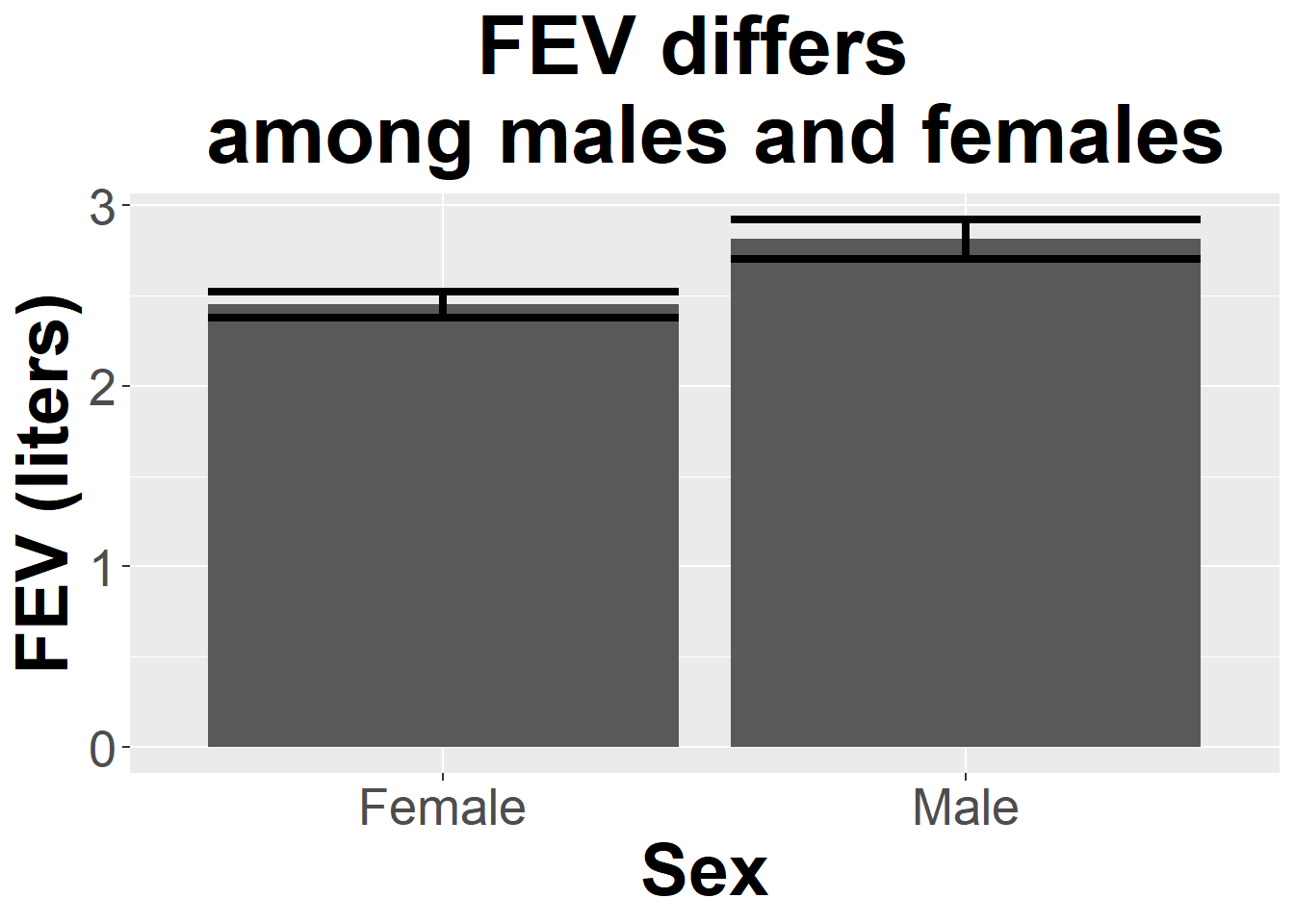
fev_gender <- lm(FEV ~ Sex, fev)
plot(fev_gender) #anova is fine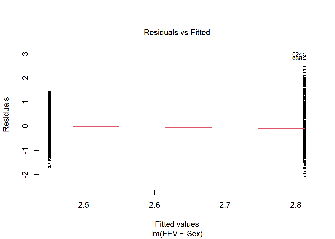
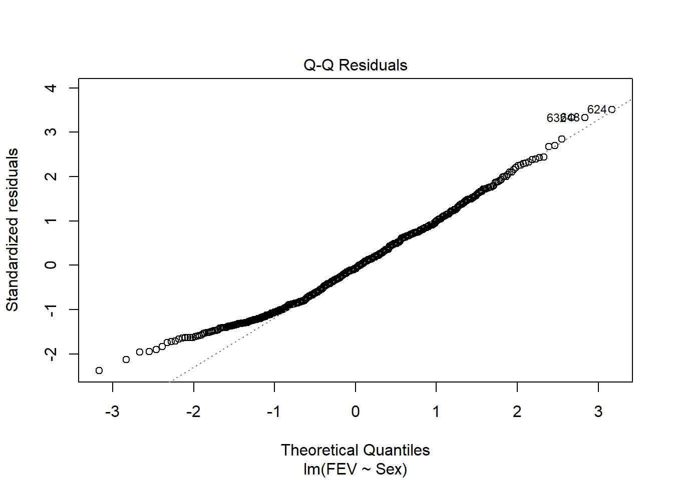
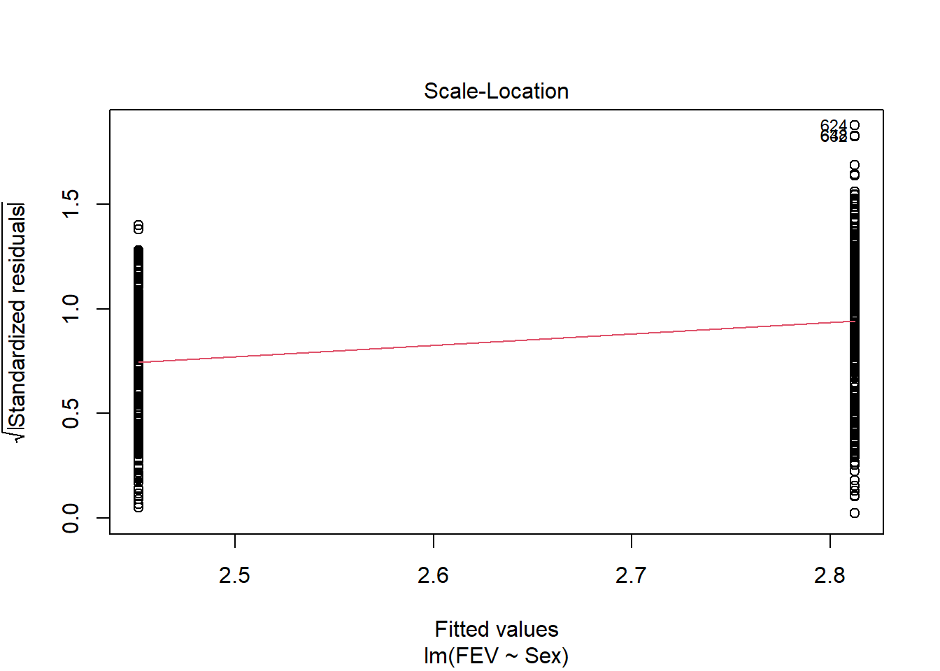
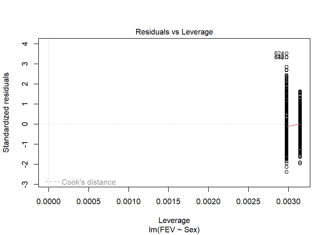
Anova(fev_gender, type = "III")Anova Table (Type III tests)
Response: FEV
Sum Sq Df F value Pr(>F)
(Intercept) 1910.62 1 2652.756 < 2.2e-16 ***
Sex 21.32 1 29.607 7.496e-08 ***
Residuals 469.60 652
---
Signif. codes: 0 '***' 0.001 '**' 0.01 '*' 0.05 '.' 0.1 ' ' 1summary(fev_gender)
Call:
lm(formula = FEV ~ Sex, data = fev)

Residuals:
     Min       1Q   Median       3Q      Max
-2.01645 -0.69420 -0.06367  0.58233  2.98055

Coefficients:
            Estimate Std. Error t value Pr(>|t|)
(Intercept)  2.45117    0.04759  51.505  < 2e-16 ***
SexMale      0.36128    0.06640   5.441  7.5e-08 ***
---
Signif. codes:  0 '***' 0.001 '**' 0.01 '*' 0.05 '.' 0.1 ' ' 1

Residual standard error: 0.8487 on 652 degrees of freedom
Multiple R-squared:  0.04344,   Adjusted R-squared:  0.04197
F-statistic: 29.61 on 1 and 652 DF,  p-value: 7.496e-08
I used an ANOVA (or linear model, or t-test, here, all the same since 2 groups!) to consider the impact of sex on FEV. This was appropriate as evidenced by the residual plots (there is no pattern in the residuals and they are normally distributed). Results indicate there is a difference among sexes (F1,652 = 29.607, p<.001). There is no need for post-hoc tests here since there are only 2 groups being considered.
Coefficients related to the groups (note female is replaced by intercept here, and the SexMale coefficient is relative to that) indicates that males have a higher FEV on average. Graphs also show this relationship.
5
The following data are human blood clotting times (in minutes) of individuals given one of two different drugs.
| Drug B | Drug G |
|---|---|
| 8.8 | 9.9 |
| 8.4 | 9.0 |
| 7.9 | 11.1 |
| 8.7 | 9.6 |
| 9.1 | 8.7 |
| 9.6 | 10.4 |
| 9.5 |
Test the hypothesis that the mean clotting times are equal for the two groups
- Estimating the variance from the data
- Using rank transform analysis
- Using a permutation test
- Using a bootstrap test
Test the hypothesis that the mean clotting times are equal for the two groups
- Estimating the variance from the data
- Using rank transform analysis
- Using a permutation test
- Using a bootstrap test
drug_b <- c( 8.8, 8.4, 7.9, 8.7, 9.1, 9.6)
drug_g <- c(9.9, 9.0, 11.1, 9.6, 8.7, 10.4, 9.5)
t.test(drug_b, drug_g)
    Welch Two Sample t-test

data:  drug_b and drug_g
t = -2.5454, df = 10.701, p-value = 0.02774
alternative hypothesis: true difference in means is not equal to 0
95 percent confidence interval:
 -1.8543048 -0.1314095
sample estimates:
mean of x mean of y
 8.750000  9.742857
Using a un-paired t-test (we learn about paired tests in the next chapter), since the experimental units were not matched and I assumed the means of each group would follow a normal distribution of unknown variance, I found a test statistics of t10.701=-2.544. This corresponds to a p-value of 0.02. This p-value is <.05, so I reject the null hypothesis that the mean clotting times are the same for the two drugs.
I could also do this using a linear model approach,but that needs a long dataframe
drug_df <- data.frame(drug= c(rep("b", length(drug_b)), rep("g", length(drug_g))), time = c(drug_b, drug_g))
drug_lm <- lm(time~drug, drug_df)
plot(drug_lm)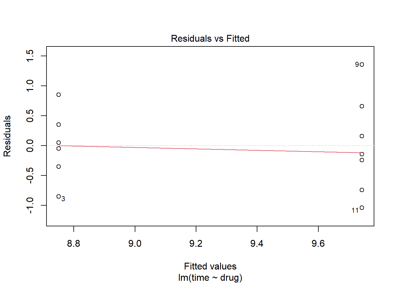
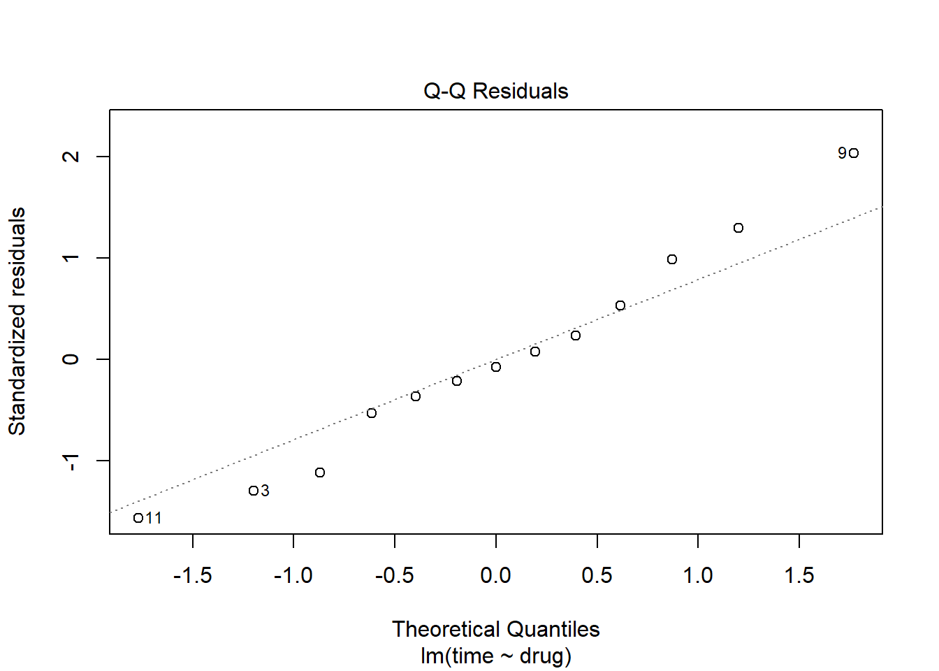
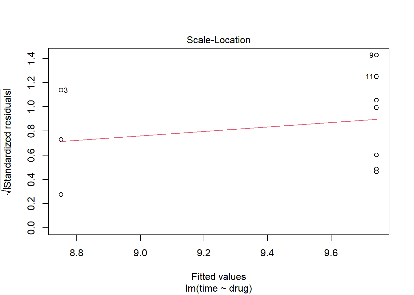
Anova(drug_lm, type="III")Anova Table (Type III tests)
Response: time
Sum Sq Df F value Pr(>F)
(Intercept) 459.38 1 884.629 7.322e-12 ***
drug 3.18 1 6.133 0.03076 *
Residuals 5.71 11
---
Signif. codes: 0 '***' 0.001 '**' 0.01 '*' 0.05 '.' 0.1 ' ' 1but that assumes variances are equal
t.test(drug_b, drug_g,var.equal = T)
    Two Sample t-test

data:  drug_b and drug_g
t = -2.4765, df = 11, p-value = 0.03076
alternative hypothesis: true difference in means is not equal to 0
95 percent confidence interval:
 -1.8752609 -0.1104534
sample estimates:
mean of x mean of y
8.750000 9.742857 - Using rank transform analysis
wilcox.test(drug_b, drug_g)Warning in wilcox.test.default(drug_b, drug_g): cannot compute exact p-value
with ties
    Wilcoxon rank sum test with continuity correction

data:  drug_b and drug_g
W = 7, p-value = 0.05313
alternative hypothesis: true location shift is not equal to 0
Using a un-paired rank-based test, which is appropriate when normality assumptions can’t be met and I assumed the means of each group would follow a similar distribution, I found a test statistics of W=7. This corresponds to a p-value of 0.05. This p-value is >.05, so I fail to reject the null hypothesis that the mean clotting times are the same for the two drugs. This is the same as
kruskal.test(time~drug, drug_df)
    Kruskal-Wallis rank sum test

data:  time by drug
Kruskal-Wallis chi-squared = 4.0221, df = 1, p-value = 0.04491
If we remove the continuity correction
wilcox.test(drug_b, drug_g, correct = F)Warning in wilcox.test.default(drug_b, drug_g, correct = F): cannot compute
exact p-value with ties
    Wilcoxon rank sum test

data:  drug_b and drug_g
W = 7, p-value = 0.04491
alternative hypothesis: true location shift is not equal to 0- Using a permutation test
require(coin) #requires data_frame
clotting <- data.frame(drug = c(rep("drug_b", length(drug_b)), rep("drug_g",
                                                                   length(drug_g))),
                       clotting = c(drug_b, drug_g))
clotting$drug <- factor(clotting$drug)
independence_test(clotting ~ drug, clotting)
    Asymptotic General Independence Test

data:  clotting by drug (drug_b, drug_g)
Z = -2.0726, p-value = 0.03821
alternative hypothesis: two.sided
Using a permutation test, which is not fully appropriate here due to small sample sizes (and that also assumes similar distributions for each group), I found a test statistics of Z=-2.0726.. This corresponds to a p-value of 0.038. This p-value is >.05, so I fail to reject the null hypothesis that the mean clotting times are the same for the two drugs.
- Using a bootstrap test
library(MKinfer)
boot.t.test(drug_b, drug_g)
    Bootstrap Welch Two Sample t-test

data:  drug_b and drug_g
number of bootstrap samples:  9999
bootstrap p-value = 0.019
bootstrap difference of means (SE) = -0.9927412 (0.353871)
95 percent bootstrap percentile confidence interval:
 -1.719048 -0.300000

Results without bootstrap:
t = -2.5454, df = 10.701, p-value = 0.02774
alternative hypothesis: true difference in means is not equal to 0
95 percent confidence interval:
 -1.8543048 -0.1314095
sample estimates:
mean of x mean of y
 8.750000  9.742857
Using a bootstrap test with 10000 samples, which is not fully appropriate here due to small sample sizes, I found a p value of 0.0047. This p-value is <.05, so I reject the null hypothesis that the mean clotting times are the same for the two drugs.
6
(Example from Handbook on Biological Statistics) Odd (stunted, short, new) feathers were compared in color to typical feathers in Northern Flickers (Colaptes auratus) (Wiebe and Bortolotti 2002) . Data is at
https://raw.githubusercontent.com/jsgosnell/CUNY-BioStats/master/datasets/wiebe_2002_example.csv
Test the hypothesis that odd and typical feathers did not differ using
- a Student’s t test and/or lm
- a rank test
- bootstrapping
Note we will return to this question next week!
- a Student’s t test and/or lm
feather <-  read.csv("https://raw.githubusercontent.com/jsgosnell/CUNY-BioStats/master/datasets/wiebe_2002_example.csv", stringsAsFactors = T)
t.test(Color_index ~ Feather, data=feather)
    Welch Two Sample t-test

data:  Color_index by Feather
t = -3.56, df = 29.971, p-value = 0.00126
alternative hypothesis: true difference in means between group Odd and group Typical is not equal to 0
95 percent confidence interval:
 -0.21579254 -0.05845746
sample estimates:
    mean in group Odd mean in group Typical
            -0.176125             -0.039000
I assumed the difference in means was normally distributed given the trait and sample size. The test resulted in a statistic of t29.971 = -3.56. This corresponds to a p-value of .001. Since the p-value is <.05, I reject the null hypothesis that feather color is the same between odd and typical feathers. Note if we assume the variances of the groups are equal (not the default for a t-test)
t.test(Color_index ~ Feather, data=feather, var.equal=T)
    Two Sample t-test

data:  Color_index by Feather
t = -3.56, df = 30, p-value = 0.001259
alternative hypothesis: true difference in means between group Odd and group Typical is not equal to 0
95 percent confidence interval:
 -0.21578936 -0.05846064
sample estimates:
    mean in group Odd mean in group Typical
            -0.176125             -0.039000
this equivalent too:
library(car)
Anova(lm(Color_index ~ Feather, data=feather), type="III")
Anova Table (Type III tests)
Response: Color_index
Sum Sq Df F value Pr(>F)
(Intercept) 0.49632 1 41.816 3.814e-07 ***
Feather 0.15043 1 12.674 0.001259 **
Residuals 0.35607 30
---
Signif. codes: 0 '***' 0.001 '**' 0.01 '*' 0.05 '.' 0.1 ' ' 1However (we’ll get to this next chapter), we should really use a blocking approach that accounts for the fact each bird was measured twice. This can be a paired t-test (note you can no longer use paired data in formula interface):
t.test(feather[feather$Feather == "Typical", "Color_index"],
       feather[feather$Feather == "Odd", "Color_index"],
       paired=TRUE)
    Paired t-test

data:  feather[feather$Feather == "Typical", "Color_index"] and feather[feather$Feather == "Odd", "Color_index"]
t = 4.0647, df = 15, p-value = 0.001017
alternative hypothesis: true mean difference is not equal to 0
95 percent confidence interval:
 0.06521848 0.20903152
sample estimates:
mean difference
       0.137125
I used a paired t-test because feathers were measured on the same bird.
I also assumed the difference in means was normally distributed given the trait and sample size. The test resulted in a statistic of t15 = -4.06. This corresponds to a p-value of .001. Since the p-value is <.05, I reject the null hypothesis that feather color is the same between odd and typical feathers. Note this equivalent too:
library(car)
Anova(lm(Color_index ~ Feather+Bird, data=feather))
Anova Table (Type II tests)
Response: Color_index
Sum Sq Df F value Pr(>F)
Feather 0.15043 1 16.5214 0.001017 **
Bird 0.21950 15 1.6072 0.184180
Residuals 0.13657 15
---
Signif. codes: 0 '***' 0.001 '**' 0.01 '*' 0.05 '.' 0.1 ' ' 1- a rank test
I could used a rank-based test if I assumed the distribution of means was symmetrical but normal.
wilcox.test(Color_index ~ Feather, data=feather)Warning in wilcox.test.default(x = DATA[[1L]], y = DATA[[2L]], ...): cannot
compute exact p-value with ties
    Wilcoxon rank sum test with continuity correction

data:  Color_index by Feather
W = 45.5, p-value = 0.001994
alternative hypothesis: true location shift is not equal to 0
which led to W=45.5, p=0.002, thus I reject the null hypothesis. However, as noted above, we will see next week we should use a paired test.
wilcox.test(feather[feather$Feather == "Typical", "Color_index"],
       feather[feather$Feather == "Odd", "Color_index"],
       paired=TRUE)
    Wilcoxon signed rank exact test

data:  feather[feather$Feather == "Typical", "Color_index"] and feather[feather$Feather == "Odd", "Color_index"]
V = 126, p-value = 0.001312
alternative hypothesis: true location shift is not equal to 0
I used a paired rank-based test because feathers were measured on the same bird. I did not assume the difference in means was normally distributed but did assume it followed a symmetric distribution. The test resulted in a statistic of V = 10. This corresponds to a p-value of .001. Since the p-value is <.05, I reject the null hypothesis that feather color is the same between odd and typical feathers.
- a binary test is only possible for paired data (so not required here, but in case you are interested…)
library(BSDA)
SIGN.test(feather[feather$Feather == "Odd", "Color_index"],
          feather[feather$Feather == "Typical", "Color_index"])
    Dependent-samples Sign-Test

data:  feather[feather$Feather == "Odd", "Color_index"] and feather[feather$Feather == "Typical", "Color_index"]
S = 3, p-value = 0.02127
alternative hypothesis: true median difference is not equal to 0
95 percent confidence interval:
 -0.24048275 -0.02331055
sample estimates:
median of x-y
       -0.114

Achieved and Interpolated Confidence Intervals:

                  Conf.Level  L.E.pt  U.E.pt
Lower Achieved CI     0.9232 -0.2400 -0.0320
Interpolated CI       0.9500 -0.2405 -0.0233
Upper Achieved CI     0.9787 -0.2410 -0.0140
I used a sign test (always paired!) because feathers were measured on the same bird. I did not assume the difference in means was normally distributed or that the differences followed a symmetric distribution. The test resulted in a statistic of s = 3. This corresponds to a p-value of .02. Since the p-value is <.05, I reject the null hypothesis that feather color is the same between odd and typical feathers.
- bootstrapping
Could be done using a non-paired approach
library(MKinfer)
boot.t.test(Color_index ~ Feather, data=feather)
    Bootstrap Welch Two Sample t-test

data:  Color_index by Feather
number of bootstrap samples:  9999
bootstrap p-value = 0.0026
bootstrap difference of means (SE) = -0.137064 (0.03707333)
95 percent bootstrap percentile confidence interval:
 -0.21012500 -0.06280938

Results without bootstrap:
t = -3.56, df = 29.971, p-value = 0.00126
alternative hypothesis: true difference in means is not equal to 0
95 percent confidence interval:
 -0.21579254 -0.05845746
sample estimates:
    mean in group Odd mean in group Typical
            -0.176125             -0.039000
or a paired approach (next chapter)
boot.t.test(Color_index ~ Feather, data=feather, paired=TRUE)
    Bootstrap Paired t-test

data:  Color_index by Feather
number of bootstrap samples:  9999
bootstrap p-value = 0.001
bootstrap mean of the differences (SE) = -0.1375529 (0.03237547)
95 percent bootstrap percentile confidence interval:
 -0.20319375 -0.07543438

Results without bootstrap:
t = -4.0647, df = 15, p-value = 0.001017
alternative hypothesis: true difference in means is not equal to 0
95 percent confidence interval:
 -0.20903152 -0.06521848
sample estimates:
mean of the differences
              -0.137125
The basic approach yield a p-value of .001, so I reject the null hypothesis that feather color is the same between odd and typical feathers.
Since feathers were measured on the same bird, I also could have used a bootstrap (10,000 samples) focused on the difference in color. This resulted in a p-value of <.001. Since the p-value is <.05, I reject the null hypothesis that feather color is the same between odd and typical feathers using this approach as well.
7
Find an example of a one-way ANOVA from a research article that is related to your research or a field of interest (hint: use Google Scholar or another search engine to search for a keyword of interest plus ANOVA). Make sure you understand the connections between the methods, results, and graphs. Briefly answer the following questions
- What is the name of the paper and who are the authors?
- What was the dependent variable?
- What were the independent variables?
- Was there a difference in mean values among the groups? If so, how did the paper address or explain this finding.
References
Wiebe, Karen L., and Gary R. Bortolotti. 2002. “Variation in Carotenoid-Based Color in Northern Flickers in a Hybrid Zone.” The Wilson Bulletin 114 (3): 393–400. http://www.jstor.org/stable/4164474.